OpenCV Tutorial Part 1: Camera Calibration
This blog post series is not a tale of a specific project technique we performed for a client, but rather a ground-up walkthrough of getting started with OpenCV. We’ve used OpenCV quite a bit in the last few years, especially in pose estimation for vision navigation, and we’ll cover some of the techniques in later posts. For now, let’s get started as if you didn’t know anything about OpenCV.
What is OpenCV?
OpenCV (Open Source Computer Vision Library) is a powerful open-source software library that provides a comprehensive suite of tools and functions for computer vision and machine learning applications. Originally developed by Intel in 1999, OpenCV was designed to accelerate the adoption of computer vision technologies by providing a robust, free-to-use library that could be easily integrated into various applications. The initial goal was to create a common infrastructure for computer vision research and to make computer vision applications more accessible and efficient. Over the years, OpenCV has grown exponentially, driven by contributions from a large and active community of developers, researchers, and engineers. This growth has transformed OpenCV into a versatile library that supports multiple programming languages, including C++, Python, and Java, and is compatible with various platforms such as Windows, Linux, Android, and macOS.
The evolution of OpenCV reflects the broader trends in the field of computer vision and machine learning. Initially focused on basic image processing tasks such as filtering, edge detection, and feature extraction, the library has expanded to include advanced algorithms for object detection, facial recognition, and 3D reconstruction. With the rise of deep learning, OpenCV has integrated support for deep learning frameworks like TensorFlow, PyTorch, and Caffe, enabling developers to leverage state-of-the-art neural network models for complex vision tasks. Additionally, OpenCV has embraced hardware acceleration, optimizing performance on GPUs and specialized hardware like FPGAs and TPUs. This adaptability and continuous evolution have made OpenCV a cornerstone in the toolkit of computer vision professionals, offering a blend of simplicity, flexibility, and performance that caters to both beginners and experts in the field.
What is OpenCV used for?
OpenCV is widely used in various real-world applications that require computer vision and image processing capabilities. In the realm of industrial automation, OpenCV plays a crucial role in tasks such as quality inspection, where it helps identify defects in products on a production line. By leveraging techniques like object detection and pattern recognition, OpenCV enables machines to perform tasks like sorting, counting, and verifying products with high accuracy and speed. In robotics, OpenCV is commonly used for vision-based navigation, enabling robots to recognize and interact with their surroundings. This includes applications like autonomous vehicles, where OpenCV is used for lane detection, traffic sign recognition, and obstacle avoidance, contributing to the development of safer and more reliable self-driving systems.
OpenCV is also extensively used in fields like healthcare, security, and entertainment. In healthcare, it aids in medical imaging by helping doctors analyze X-rays, MRIs, and other scans to detect anomalies such as tumors or fractures. In the security domain, OpenCV is employed in surveillance systems for tasks like motion detection, facial recognition, and license plate recognition, enhancing the effectiveness of monitoring and threat detection. The entertainment industry leverages OpenCV in augmented reality (AR) and virtual reality (VR) applications, where it helps track and overlay digital content onto the real world in real-time. Additionally, OpenCV is utilized in the development of interactive installations, video games, and visual effects, making it a versatile tool in creating immersive and engaging experiences.
What has AlphaPixel used OpenCV for?
AlphaPixel has used OpenCV in many different contexts over the years. We’ve used it for a variety of fiducial marker tracking tasks, from Augmented Reality smartphone/tablet applications, to robotic vision navigation. We’ve used it for realtime segmentation of objects in a video feed, as well as combining it machine learning tools like YOLO and Segment Anything. We’ve used feature-extraction and tracking methods like SIFT and SURF to track known and unknown non-fiducial entities. We’ve done a variety of stereo-camera operations, and combined it with specialty vision cameras like the Microsoft Kinect and the OAK-D depth camera. We’ve combined OpenCV with Unreal Engine, OpenSceneGraph and a variety of head mounted VR/AR displays like the Oculus series and the Meta Quest.
How do I get started with OpenCV?
Getting started with OpenCV is relatively straightforward, especially given its broad support for multiple programming languages and platforms. If you’re new to OpenCV, the first step is to install the library on your development environment. For Python users, this can be done easily using pip, the package installer for Python, with the command pip install opencv-python. C++ developers can install the precompiled binaries from the official OpenCV website or build the library from source, which allows for greater customization and optimization. OpenCV is also in vcpkg, Conan and homebrew. I’m going to be working in Windows and Python here. We may do a later post on replicating the same work in C++.
What prerequisites do I need for Camera Calibration with Python in OpenCV
- Python 3.x (and PIP)
- Numpy
- OpenCV for Python
- A camera that can produce digital images and a way to display or print the calibration chessboard, or some sample digital images (which we provide)https://alphapixeldev.com/wp-content/uploads/2024/08/Cleaned.zip
Steps to install Python+OpenCV in Windows
- Install Python
- https://www.python.org/downloads/windows/
- Download and run the Installer. Make sure you have Python in your PATH so it can be invoked from your preferred command-line shell (CMD, PowerShell, Terminal)
- Install PIP
- https://www.geeksforgeeks.org/how-to-install-pip-on-windows/
- Download and save the file from https://bootstrap.pypa.io/get-pip.py
-
python get-pip.py
- (optionally) Create a virtual environment
- https://docs.python.org/3/library/venv.html
- This allows you to have a custom environment for this project, which contains specific versions of the tools and libraries we are using
-
python -m venv /path/to/new/virtual/environment
- Then change directory to /path/to/new/virtual/environment and work from there.
- Install Numpy
- https://numpy.org/install/
-
pip install numpy
- Install OpenCV
- pip install opencv-python
- Test the OpenCV installation
-
python
-
>>>import cv2
-
>>>print(cv2.__version__)
-
Here’s a blog post entirely about installing Python and OpenCV on Windows.
What’s the first step after installing OpenCV?
The first step to get going with OpenCV is to create some input images to perform camera calibration. OpenCV performs computer vision tasks, and a large portion of those tasks require a calibrated camera in order to understand the relationship between pixels in an image and their positions in the real-world space the camera can view. This is necessary in order to perform 3d and spatial calculations on the image. If all you need to do is basic 2d operations (segmenting, etc) on an image, camera calibration may not be necessary. The interesting tasks we want to do involve 3d space, so we will start with camera calibration.
What is Camera Calibration in OpenCV?
Camera calibration is a crucial step in most computer vision tasks, as it allows you to determine the intrinsic parameters of a camera, which are essential for accurately interpreting the geometry of the scene being captured. Camera calibration involves estimating the camera’s internal parameters, such as the focal length, optical center (principal point), and lens distortion coefficients. These parameters describe how the camera projects 3D points in the world onto a 2D image plane. The goal of camera calibration is to correct distortions and improve the accuracy of measurements and image processing tasks, such as 3D reconstruction, object detection, and augmented reality applications. Here’s an official OpenCV camera calibration guide:
https://docs.opencv.org/3.4/dc/dbb/tutorial_py_calibration.html
How does one perform Camera Calibration in OpenCV?
In practice, camera calibration in OpenCV is typically performed using images of a known calibration pattern, such as a “chessboard”. The process begins by capturing multiple images of the calibration pattern from different angles and distances. These images are then processed to detect the corners of the pattern’s features. Once these points are identified in each image, OpenCV’s cv2.calibrateCamera() function is used to estimate the camera’s intrinsic parameters by solving a series of equations that relate the 2D image points to their corresponding 3D world points. The output of this process includes the camera matrix, distortion coefficients, (and rotation and translation vectors). These calibration parameters can then be used to undistort images, correct perspective, and accurately interpret spatial relationships in the scene.
Capturing pictures for Camera Calibration in OpenCV
When performing camera calibration in OpenCV, you need to adhere to several preconditions to ensure accurate and reliable results. These preconditions relate to the quality and consistency of the images used in the calibration process, as well as how the images are captured and handled before they are processed by OpenCV. Meeting these preconditions helps to minimize errors in the calibration process and leads to more precise determination of the camera’s intrinsic and extrinsic parameters.
Resolution, Clarity, Noise, and Contrast
The images used for calibration should have high resolution, be clear, and have minimal noise. Sharp images with good contrast between the calibration pattern and the background are crucial for accurately detecting and identifying the features of the pattern, such as corners or circles. Avoid low-light situations that make the camera crank up the electronic exposure, resulting in digital grain noise. Also, avoid heavy JPG compression – set as high of an image quality as you can if it’s adjustable. You can shoot DNG or other RAW format and convert to PNG to avoid introducing compression artifacting, but for the most part it shouldn’t be a problem. If you re capturing using OpenCV itself (from a camera connected to your computer, eg a webcam or other dedicated camera), make sure to configure it for the resolution you intend to use during actual vision operations.
EXIF Data Is NOT Needed or Useful to OpenCV
When capturing images for calibration, the EXIF data (which includes information like exposure settings, camera model, lens intrinsics and date) is not necessary for the calibration process in OpenCV. OpenCV focuses purely on the pixel data to perform the calibration, so any EXIF information is irrelevant and does not contribute to the accuracy of the results. Other tools may find the lens intrinsics useful and OpenCV CAN access the EXIF data with check_exif(), but the calibration process doesn’t rely on it. (Sidebar: Here’s a cool article on using EXIF data in OpenCV)
No Cropping or Other Spatial Altering of the Image
Avoid cropping or any other spatial alterations, such as resizing, rotating, or warping, of the images used for calibration. Any such changes can distort the calibration pattern and lead to inaccurate detection of the pattern features, which will, in turn, compromise the calibration results.
Consistent Zoom
When capturing images for calibration, the zoom level of the camera MUST remain consistent across all images. Changes in zoom can alter the apparent shape and distortion of the calibration pattern in the images, which WILL ruin the accuracy of the calibration parameters (because the system intrinsics are different at different zoom levels). Maintaining consistent zoom ensures that the relationship between the 3D world points and their 2D projections remains stable. If it is necessary to handle zooming, you will need to perform the calibration process using multiple sets of images, each taken at different zoom, and construct an interpolation process for blending between intrinsics models at the nearest zoom levels.
Sufficient Number and Variety of Images
A successful calibration requires a sufficient number of images that cover a wide range of orientations and positions of the calibration pattern within the camera’s field of view. This variety ensures that the calibration process accounts for different perspectives and angles, which is crucial for accurately estimating the camera’s intrinsic parameters. The more diverse the images, the more reliable the calibration will be, as it allows the algorithm to robustly handle different viewing conditions.
How do I generate and print the OpenCV Calibration Chessboard?
Generating and printing an OpenCV calibration chessboard is a straightforward process that involves creating a standard checkerboard pattern using OpenCV’s built-in tools or by downloading one from an online pattern creator. The chessboard pattern is a grid of black and white squares, with the most common sizes being 6×9 or 7×10 squares (excluding the outer edges, which are not counted). I’m including a trustworthy 10×7 chessboard PDF below.
To generate the pattern locally the cv2.drawChessboardCorners() function creates the grid and then it can be saved as an image file, such as a PNG or PDF. Once generated, it’s important to print the chessboard pattern on a flat, non-glossy surface using a high-resolution printer to ensure clarity and sharpness. The printed chessboard should then be affixed to a rigid backing to prevent any warping or bending during the calibration process, as even slight distortions can affect the accuracy of the calibration. Additionally, make sure that the printed pattern is not scaled or resized during printing, as this would alter the square sizes and compromise the calibration results.
Here is a PDF of a landscape-format A4 10×7 landscape chessboard with 25mm squares. I chose this size because it will fit without scaling or cropping anything important on a US Letter or ISO A4 sheet of paper that most printers can print.
When you go to print this, make sure you choose the proper scaling in your viewing/printing application. When I printed in Adobe Acrobat under Windows, the print dialog looked like this.
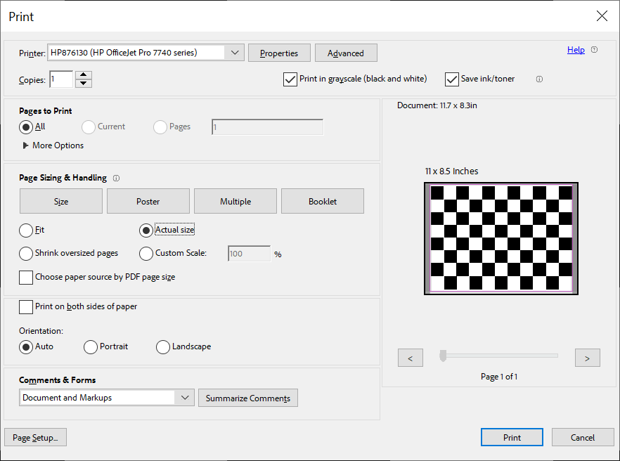
Make sure to select Landscape orientation and Actual Size or 100% or whatever your platform uses. You do NOT want to fit or shrink the printout. If your printer can’t print all the way to the margins (most can’t) it’s ok. Let it crop the edges as long as the scale stays 100%. If you look at the example image from the OpenCV Python calibration tutorial, OpenCV doesn’t USE the outer edges of the chessboard, it will only identify feature points where four FULL squares (two black, two white) are completely visible.
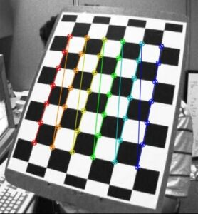
This is NOT my chessboard, it’s a 9×6 of some sort with 7×6 useable.
Credit https://docs.opencv.org/3.4/dc/dbb/tutorial_py_calibration.html
How do I photograph the OpenCV Calibration Chessboard?
Ok, now that this has printed, let’s go photograph it. Where should we do this? Well, based on the suggested preconditions above, we want somewhere well-lit where you can set the target down and move around it and take photos from many angles. It’s best that you not cast a shadow on the target while taking photos, so overhead light is best. You WILL however, want to take a photo from directly overhead, so if you’re using an interior environment with an overhead light, make sure you can get above without blocking the light.
In my case, for expediency, I did not mount the target, I just printed it on regular letter-sized paper and set it on a flat surface. For greater precision, I should do a better job, but I’m also trying to make this as easy for you, the reader, to replicate with minimal supplies and effort. If my lame attempt at calibration works, yours should too!
I photographed the target outdoors, on a concrete patio, with minimal other clutter visible. I utilized morning (side) natural light to avoid casting a shadow from above. White balance and color correction shouldn’t matter. The patterns in the concrete should not interfere too much with the chessboard corner detection. I prefer to not have too much clutter in my images, but in reality the chessboard corner detection is very robust and as long as you’re not taking photos on the vinyl tiled floor of a 50s diner, you should be fine.
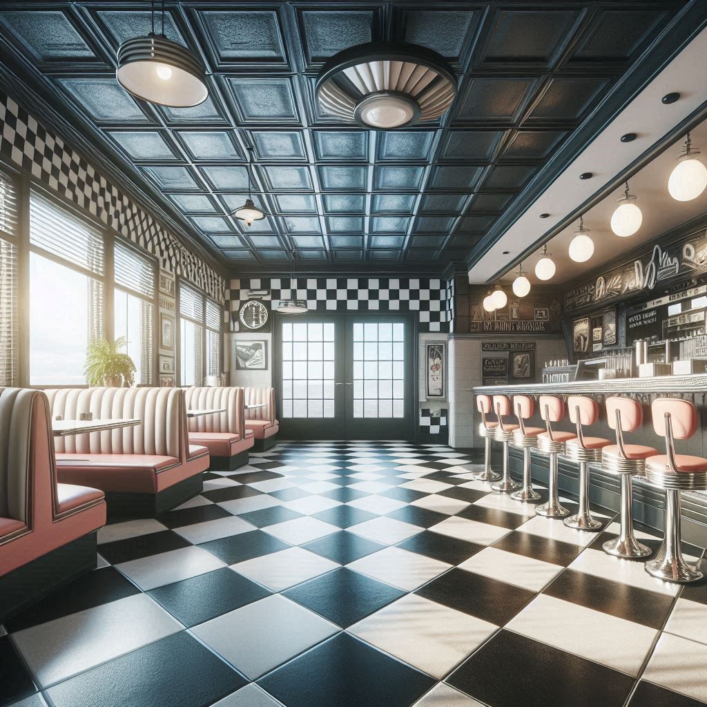
This would be a terrible place to calibrate, especially since it’s weird generative AI and doesn’t exist.
Credit: Microsoft Bing Image Creaator.
If you’re using a smartphone to take the photos, make sure you keep it in the same orientation (portrait versus landscape) as you plan to do OpenCV work in, and make sure the images don’t come out rotated weird or upside down. Smartphones try to smart-flip you images to be “upright” depending on which way the phone’s accelerometer senses gravity, and write EXIF data that note which end is up. OpenCV doesn’t know anything about gravity and wants the camera in the same orientation at all times. You can also keep your phone/camera in a fixed position and move your chessboard around in front of it. My unmounted paper chessboard was too floppy to do this.
How many calibration images are recommended for OpenCV camera calibration?
it is generally recommended to use at least 10 to 20 calibration images to obtain accurate results. These images should capture the calibration chessboard pattern from different angles, distances, and orientations to ensure that the camera’s intrinsic parameters are well estimated. The more varied the images, the better the calibration will be, as this variety helps to cover a wide range of perspectives, reducing the potential for errors and increasing the robustness of the calibration process. However, using more than 20 images can further improve accuracy, especially if you are calibrating a camera with complex distortion characteristics.
In our case, I took 20 photos at different distances, angles and perspectives. I’ve removed all the metadata I could from these using https://jimpl.com/ for privacy and to prove it’s not needed.
Here’s a contact sheet of all 20 images. (A couple of these are upside down, I fixed this before using them later).
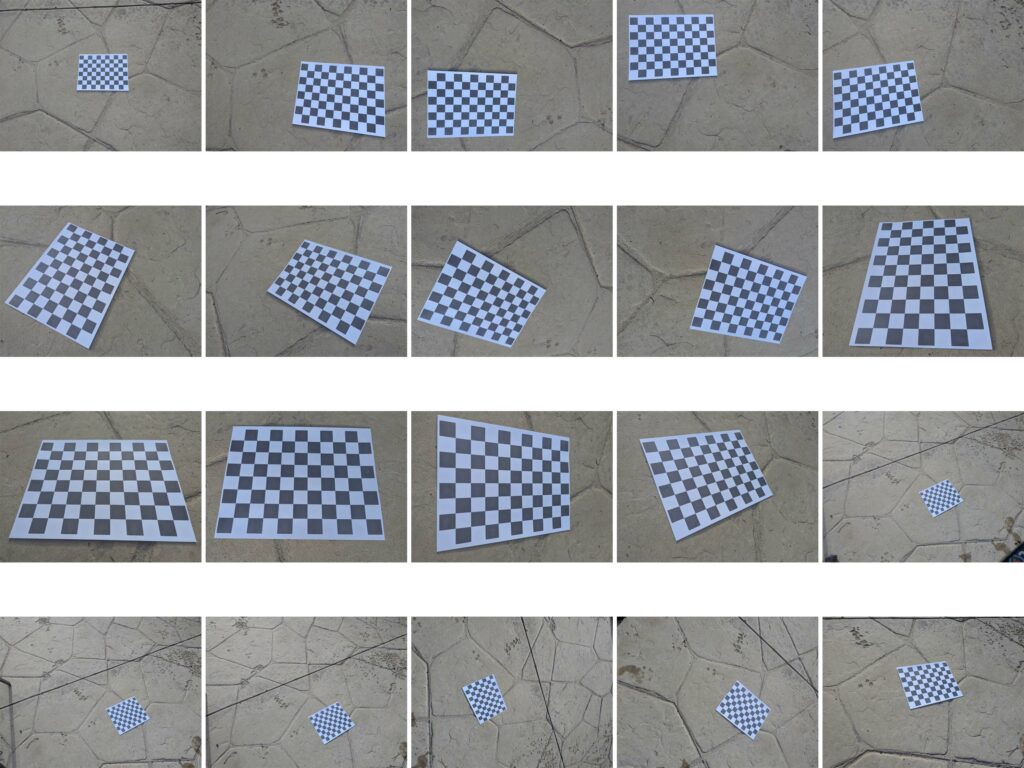
You can download my sample OpenCV Calibration images here.
You can check and make sure if your chessboards in your calibration images cover the image area sufficiently by layering them all together. Here, I used Photoshop to select-by-color-range only the white (making the black and concrete transparent), and layer the images atop one another, using a Lighten blend mode and a 25% opacity on each layer.
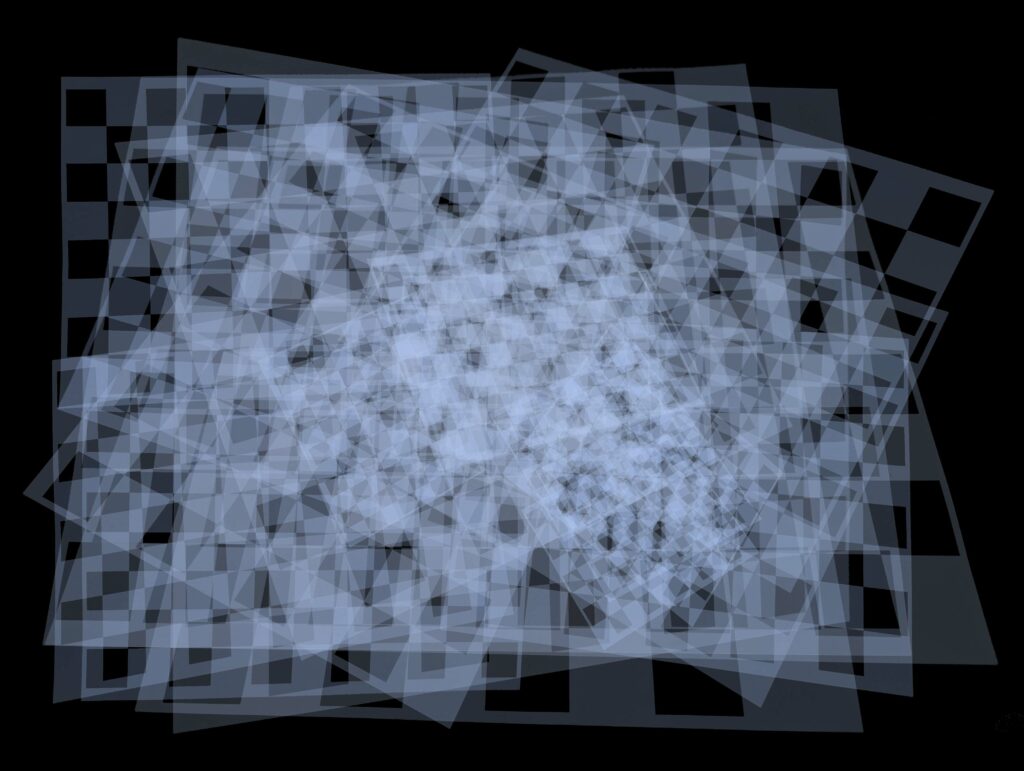
This makes it clear that we have pretty good coverage. I might have been more careful to get the chessboard into every corner, but we can assume that precision should be fairly good in the center of the image. You need to ensure all 10×7 (or however-many) intersections are visible in every calibration image.
Now, let’s calibrate!
How do I perform the actual OpenCV Camera Calibration step?
The steps you need to do in Python are generally these:
-
- Prepare the process
- For each image
- Load the image
- Convert to Grayscale
- Find the chessboard corners
- Refine the location of the corners
- Add the corners to the dataset
- Perform calibrateCamera()
- Optionally, report or save (serialize) the calibration data for later use
Let’s start with some code to load images and find corners. I’ve expanded and added comments, so it should be pretty self-explanatory.
# derived from https://docs.opencv.org/4.x/dc/dbb/tutorial_py_calibration.html
# and https://learnopencv.com/camera-calibration-using-opencv/
# all OpenCV source code copyrights respected

import numpy as np
import cv2 as cv
import glob

# prepare the process

# define the dimensions of chessboard in square=intersections (not real-world size of each square)
# the chessboard dimensions are the number of INTERSECTIONS BETWEEN squares, not the number
# of SQUARES between INTERSECTIONS. So a 10x7 chessboard has 11 squares across and 8 squares high
CHESSBOARD = (10,7)

# width (in pixels) of the user's preferred preview window size, for convenience in resizing data being displayed to fit
SCREENWIDTH = 1000

# define termination criteria for cornerSubPix refinement
# 0.001 is the accuracy (called Epsilon) and 30 is the max iteration count
criteria = (cv.TERM_CRITERIA_EPS + cv.TERM_CRITERIA_MAX_ITER, 30, 0.001)

# prepare object points, like (0,0,0), (1,0,0), (2,0,0) ....,(9,6,0)
objp = np.zeros((CHESSBOARD[0]*CHESSBOARD[1],3), np.float32)
objp[:,:2] = np.mgrid[0:CHESSBOARD[0],0:CHESSBOARD[1]].T.reshape(-1,2)

# Arrays to store object points and image points from all the images.
objpoints = [] # 3d point in real world space
imgpoints = [] # 2d points in image plane.

images = glob.glob('*.jpg')

for fname in images:
    img = cv.imread(fname)
    gray = cv.cvtColor(img, cv.COLOR_BGR2GRAY)

    # Find the chess board corners
    # If desired number of corners are found in the image then ret = true
    # we are passing the two optional args (which default to true):
    # AdaptiveThresh Use adaptive thresholding to convert the image to black and white, rather than a fixed threshold level (computed from the average image brightness). default true.
    # NormalizeImage Normalize the image gamma with cv.equalizeHist before applying fixed or adaptive thresholding. default true.
    ret, corners = cv.findChessboardCorners(gray, CHESSBOARD, cv.CALIB_CB_ADAPTIVE_THRESH + cv.CALIB_CB_NORMALIZE_IMAGE)

    # If found, add object points, image points (after refining them)
    if ret == True:
        objpoints.append(objp)

        # refine the corner location into sub-pixel decimal coordinates
        # by analyzing a window of surrounding pixels and computing gradients to
        # estimate where the intersectino fell between pixel centers
        corners2 = cv.cornerSubPix(gray,corners, (11,11), (-1,-1), criteria)
        imgpoints.append(corners2)

        # Draw and display the corners
        cv.drawChessboardCorners(img, CHESSBOARD, corners2, ret)

        # resize image to fit a reasonable screen size if overly large
        origHeight, origWidth = img.shape[:2] # get current image dimensions
        displayRescaleFactor = SCREENWIDTH / origWidth # calculate how those relate to the preferred size
        if displayRescaleFactor < 1.0: # is it too big?
            # resize the preview image down to not be awkward
            img = cv.resize(img, (0, 0), fx = displayRescaleFactor, fy = displayRescaleFactor, interpolation = cv.INTER_AREA) # cv.INTER_AREA makes for cleaner downsize of lines

        cv.imshow('OpenCV Calibration', img)
        cv.waitKey(100)

cv.destroyAllWindows()
Put this code in the same folder as the calibration images and run it
python alphapixel-opencv-camera-chessboard.py
It will look for all jpg images in the current folder (you can change the file extension on line 31).
It should load each image in turn and if successful, display a window like this for each photo for a short time. These are fairly large images, if you find it’s going to slowly, you can bulk resize them all down to a more convenient size. Just make sure they’re all the SAME size and you don’t crop or stretch them.
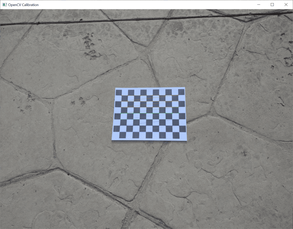 Calibration image with chessboard corners drawn on top of it.
(Yes, I need a new concrete coating.)
Credit: The author.
Great! We’ve identified the chessboard corners. Now we need to use them to create a calibration profile for the camera intrinsics. We do this with calibrateCamera().
We do this with one simple OpenCV call.
ret, mtx, dist, rvecs, tvecs = cv.calibrateCamera(objpoints, imgpoints, gray.shape[::-1], None, None)
It takes the input object points (objpoints) and image points (imgpoints) identified in the chessboard corners extraction above, along with the image dimensions of one of the images (gray). It returns an RMS error value (ret), an Intrinsic Camera Matrix (mat), Lens Distortion Coefficients (dist), Rotation Vectors (rvecs) and Translation Vectors (tvecs).
The ret RMS Error value tells you how well the algorithm was able to construct a model of the camera that can reconstruct the input images mathematically. The way to determine if the calibrateCamera() function has been successful is to evaluate the reprojection error (ret), which measures the difference between the observed image points (detected corners in the calibration images) and the projected points (those calculated using the estimated camera parameters). After running the calibration, the function returns a mean reprojection error measured in pixels.
A lower reprojection error indicates a more accurate calibration. As a general rule, a reprojection error of less than 0.5 pixels is considered good, while a value below 1 pixel is generally acceptable for many applications. However, the acceptable error margin will vary depending on the specific requirements of your application. In our case, using very high-resolution (4k horizontally) camera images, we’re accepting up to 2 pixels of error as success, since our high-res camera has pixels of VERY small angular arc extant. In reality, you should probably decide on the error threshold by computing the pixel extent that corresponds to the minimum arc error you desire.
I test and print the RMS like this:
if ret < 2.0:

print ("Calibration successful, RMS re-projection error: " + str(ret))
With these test images, I get:
Calibration successful, RMS re-projection error: 1.686471789897741
These photos were taken on the Pixel 6 Pro primary back camera that is said to be a 24mm equivalent. A 24mm lens focal length comes out to about 73.7 degrees horizontal FOV. So, if we divide our 73.7 degree FOV by our 4080 pixels wide, we get about 0.018 arc degrees per pixel. There are 60 arc minutes and 3600 arc seconds in each arc degree, so multiplying by 3600 tells us we have about 65 arc seconds per pixel. Multiplying that time our RMS of 1.686471789897741 pixels, that gives us a registration accuracy of 109.67 arc seconds. How big is one arcsecond? Really small. “One arcsecond on the moon is 1.87km”. So, when viewed from Earth, one arcsecond of angular extent across your vision is about the size of a 2km diameter crater on the moon. That’s small enough you probably can’t even pick one out with the naked eye.
Now, for the final steps, I’m going to print the various pieces of data produced by the calibration process:
print ("Intrinsic Camera Matrix")

print (mtx)

print ("Lens Distortion Coefficients")

print (dist)

print ("Rotation Vectors")

print (rvecs)

print ("Translation Vectors")

print (tvecs)
Which looks like:
Intrinsic Camera Matrix

[[3.02713482e+03 0.00000000e+00 2.03524083e+03]

[0.00000000e+00 3.02779565e+03 1.47234601e+03]

[0.00000000e+00 0.00000000e+00 1.00000000e+00]]

Lens Distortion Coefficients

[[ 6.12753792e-02 -2.45608881e-01 -1.36944284e-03  3.84787851e-05

4.25470503e-01]]

Rotation Vectors

(array([[-0.31951313],

[ 0.06836755],

[ 0.00774529]]), array([[-0.27825901],

[ 0.16040039],

[ 0.10069697]]), array([[ 0.24276694],

[ 0.14879323],

[-3.08166111]]), array([[-0.12244472],

[-0.10481553],

[-0.06082787]]), array([[-0.29579925],

[-0.10194463],

[-0.16470882]]), array([[-0.35001373],

[-0.29166003],

[-1.08863384]]), array([[-0.41584261],

[ 0.40202745],

[ 0.49811303]]), array([[-0.23300959],

[ 0.37909038],

[ 0.49128026]]), array([[-0.20236031],

[ 0.2732261 ],

[ 0.28225876]]), array([[-0.4816043],

[-0.325154 ],

[-1.5271542]]), array([[-0.57291554],

[ 0.03087995],

[ 0.01780841]]), array([[ 0.02772962],

[-0.45759713],

[-3.09709793]]), array([[-0.02240767],

[-0.4304927 ],

[-0.0025043 ]]), array([[-0.29867433],

[-0.5082198 ],

[-0.36033136]]), array([[-0.45187787],

[-0.29040647],

[-0.48116866]]), array([[-0.49980195],

[-0.25954281],

[-0.448516  ]]), array([[-0.49787403],

[-0.28918766],

[-0.4827065 ]]), array([[-0.09994768],

[-0.52022216],

[ 1.13002123]]), array([[-0.25066539],

[-0.24810151],

[ 0.66166555]]), array([[-0.45133301],

[-0.35836523],

[-0.28574408]]))

Translation Vectors

(array([[-3.9286303 ],

[-3.04094072],

[34.97514136]]), array([[ 0.19760744],

[-0.27660812],

[21.17598239]]), array([[-0.76012951],

[ 7.38165793],

[20.71808892]]), array([[-10.49551915],

[ -6.29935626],

[ 19.94104902]]), array([[-11.04843066],

[  0.89877802],

[ 20.48605056]]), array([[-7.0656249 ],

[ 1.95333468],

[14.01594079]]), array([[ 0.05139224],

[-3.81128923],

[19.80697441]]), array([[ 0.45139735],

[-6.45001777],

[18.69678681]]), array([[-6.85621565],

[-5.67115255],

[17.97603225]]), array([[-3.2638071 ],

[ 3.29202759],

[ 9.84700979]]), array([[-4.23022714],

[-2.80912511],

[13.05537802]]), array([[ 4.08392746],

[ 2.45234821],

[10.30603225]]), array([[-3.75004387],

[-3.04175636],

[10.02637854]]), array([[-5.01611299],

[-2.70292943],

[12.72998311]]), array([[ 0.19663272],

[ 3.29732721],

[44.98668066]]), array([[ 2.99797702],

[ 6.85377009],

[45.78685954]]), array([[ 2.11498324],

[ 8.67515812],

[43.25661165]]), array([[-5.71196725],

[-2.56418904],

[39.56755449]]), array([[ 4.61711876],

[-0.41423407],

[34.77651634]]), array([[-3.646092  ],

[-3.10204433],

[28.40983321]]))
What is the ‘mat’ intrinsic camera matrix?
The intrinsic matrix ‘mat’ contains the focal lengths (fx, fy) and the principal point (optical center (cx,c y)) of the camera. Fundamentally this allows you to forward and reverse project points between the 3d world coordinate space in front of the camera, and a 2d camera “film” or “sensor” plane (plus a distance value).
The intrinsic matrix models a perfect pinhole camera, which is an idealized camera model that assumes light rays pass through a single point (the pinhole) and project onto an image plane. In this model, the camera has no lens distortions, and the relationship between the 3D world points and their 2D image projections is purely linear. The intrinsic matrix encapsulates the internal characteristics of the camera, such as:
Focal lengths fx, fy: These represent the scaling factors in the x and y directions of the image plane.
Principal point/optical center cx, cy: This is the point where the optical axis intersects the image plane, ideally located at the center of the image. In a perfect camera, this should be at the center, implying the lens is perfectly mounted in front of the sensor or film. In practice, real cameras sometimes do this imperfectly. We’ve worked with a USD $300,000 imager that had this grossly offset.
Skew coefficient: In most cases, this is zero, assuming that the image axes are perpendicular, as they would be for most normal cameras. Non-zero skew coefficients in the intrinsic matrix can be representative of a tilt-shift camera design, although it is more broadly a measure of any non-perpendicularity between the image axes.
Taken together, these make up the 3×3 matrix that is the ‘mat’ object.
Intrinsic Camera Matrix

[[3.02713482e+03 0.00000000e+00 2.03524083e+03]

[0.00000000e+00 3.02779565e+03 1.47234601e+03]

[0.00000000e+00 0.00000000e+00 1.00000000e+00]]
What is the ‘dist’ lens distortion?
Real physical lenses that aren’t perfect mathematical pionholes introduce distortions that deviate from the ideal model. These distortions arise due to the shape and construction of the lens, and they must be accounted for to accurately project 3D points onto the 2D image plane (and back).
In OpenCV, lens distortion is typically modeled using two types of distortions:
- Radial Distortion: This distortion causes straight lines to appear curved, especially near the edges of the image. It is described by a set of coefficients (k1, k2, k3) in the distortion model. The effect is more pronounced in wide-angle lenses.
- Tangential Distortion: This distortion occurs due to the lens being slightly misaligned relative to the image plane, causing some regions of the image to be displaced more than others. It is modeled using coefficients (p1, p2).
These make up the 5 elements of the ‘dist’ object.
Lens Distortion Coefficients

[[ 6.12753792e-02 -2.45608881e-01 -1.36944284e-03  3.84787851e-05

4.25470503e-01]]
These distortion coefficients are part of the calibration process and are used to correct the captured images, making them as close as possible to the ideal pinhole model. By combining the intrinsic matrix (which assumes a perfect pinhole camera) and the distortion coefficients (which model the real-world lens imperfections), OpenCV can accurately represent and correct the camera’s behavior, enabling precise computer vision tasks.
What are the tvecs and rvecs?
Tvecs and rvecs are the translation vectors and rotation vectors, respectively, that express where the chessboard was found in 3d space, relative to the camera’s sensor’s optical center. An open question I haven’t really found a satisfactory answer to is what UNITS these translation vectors are in. You see, at this point, OpenCV has never been told what the real-world dimensions of the chessboard were, only that it has a certain number of intersections wide, and high. So, it has no way to tell if the chessboard is on a single sheet of paper, or whether it’s been scaled up double to cover an 11”x17” sheet, or even larger (or smaller). Optically and mathematically, a big flat object far away calculates the same as a small one close up (a boon to filmmakers using miniatures for effects). So, it is my belief that these vectors are probably expressed in units of chessboard square size. I’ll demonstrate why this is, next.
What do the tvecs values look like?
We can convert the text dump of the tvecs object into a CSV and it looks like this

-3.9286303,-3.04094072,34.97514136,

0.19760744,-0.27660812,21.17598239,

-0.76012951,7.38165793,20.71808892,

-10.49551915,-6.29935626,19.94104902,

-11.04843066,0.89877802,20.48605056,

-7.0656249,1.95333468,14.01594079,

0.05139224,-3.81128923,19.80697441,

0.45139735,-6.45001777,18.69678681,

-6.85621565,-5.67115255,17.97603225,

-3.2638071,3.29202759,9.84700979,

-4.23022714,-2.80912511,13.05537802,

4.08392746,2.45234821,10.30603225,

-3.75004387,-3.04175636,10.02637854,

-5.01611299,-2.70292943,12.72998311,

0.19663272,3.29732721,44.98668066,

2.99797702,6.85377009,45.78685954,

2.11498324,8.67515812,43.25661165,

-5.71196725,-2.56418904,39.56755449,

4.61711876,-0.41423407,34.77651634,

-3.646092,-3.10204433,28.40983321
Now, my chessboard was printed with squares that seem to be about one inch on a side. So, that means our tvecs coordinates also would be close to an inch. So, our tvecs Z values, which range from about 10 to 45 units would reflect about one foot to four feet away while taking the photos. Referring to the contact sheet, this looks like a plausible interpretation.
Here’s a 2D plot of the XY values as well:
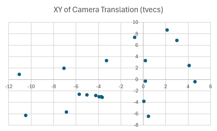 See those dots close together at around -4, -3? I believe those correspond with the last/rightmost image in the third row of the contact sheet and the two leftmost images in the fourth row. These were all taken in roughly the same spot, just reframing the rotations.
We could if we wanted, come up with a way to plot all of these camera poses in 3d, but for this article, we’ll stop here.
Next time we’ll demonstrate how to store and recall the camera calibration parameters, compute camera pose relative to one or more known markers (often called fiducial markers) and use AprilTag detection.
Here is the AlphaPixel OpenCV Camera Calibration Code in both variants — the chessboard-identifier and the full camera calibration Python scripts.
AlphaPixel solves difficult problems every day for clients around the world. We develop computer graphics software from embedded and safety-critical driver level, to VR/AR/xR, plenoptic/holographic displays, avionics and mobile devices, workstations, clusters and cloud. We’ve been in the computer graphics field for 35+ years, working on early cutting-edge computers and even pioneering novel algorithms, techniques, software and standards. We’ve contributed to numerous patents, papers and projects. Our work is in open and closed-source bases worldwide.
People come to us to solve their difficult problems when they can’t or don’t want to solve them themselves. If you have a difficult problem you’re facing and you’re not confident about solving it yourself, give us a call. We Solve Your Difficult Problems.
