AlphaPixel is always looking towards the next cutting edge of computer graphics and performance computing. In 2023, a new technique for creating realistic scenes from sparse photos debuted, called Gaussian Splats.

Welcome to our more than comprehensive guide to Gaussian Splats. If you’re reading this it’s probably because you have heard of Gaussian Splats and have a LOT of questions. What are Gaussian Splats? What are Gaussian Splats used for? How do you create Gaussian Splats? How do you view Gaussian Splats? What are Spherical Harmonics and how are they used by Gaussian Splats? What are the advantages and disadvantages of Gaussian Splats compared to polygonal photogrammetry and radiance fields like NeRFs? Who actually was Carl Friedrich Gauss and why do we care? Ok, you probably didn’t ask that last one.

What are Gaussian Splats?

We’re going to start at the beginning, and explain as thoroughly as we can, without too much heavy math or tech. Let’s decompose the words, “Gaussian Splat” and unpack what they mean together.

What are Splats?

Splats have been a rendering technique for years, mostly in the realm of texturing. Texture splatting is a method of blending two different material appearances together based upon a third, blending mask texture.

By Simeon87 – Own work, CC BY-SA 3.0, https://commons.wikimedia.org/w/index.php?curid=4371291

What does Gaussian mean?

Ok, so what’s Gaussian got to do with it (with apologies to Tina Turner)?

Wikipedia again explains (with a lot of math) that it’s a function that has little value at the edges, and a rounded peak of value in the middle. In 2D it creates a nice round blended spot of value in the middle of the domain of influence.

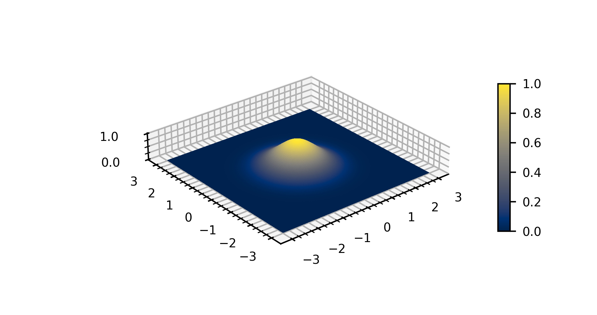
By Kopak999 – Own work, CC BY-SA 4.0, https://commons.wikimedia.org/w/index.php?curid=97678049

Gaussian Splats Explained

So, taken together, a Gaussian Splat is a thing that blends textures together using a Gaussian function to modulate where the texture is (and isn’t). Which is a pretty good description of the point-blob bits that make up a Gaussian Splats scene. A single 3D Gaussian is a spheroid-shaped blob (it can be stretched different amounts on its X, Y and Z axes) with texturing that is most opaque in the center and fades out towards the edges of the Gaussian. Interestingly, the texture is a view-dependent Spherical Harmonic, which means it can have a different appearance depending on which direction it’s observed from.

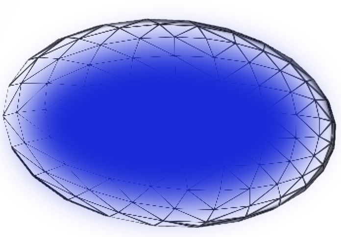
A 3d ellipsoid splat textured with monocolor Gaussian texture blend falloff.
By the author, Chris Hanson.

So, we’re done? You understand everything about Gaussian Splats now? Oh, yeah, there’s more. Like, how did we get here?

Gaussian splats are a new way of rendering what has been known previously as a Radiance Field. Same as it ever was. So, let’s talk about Radiance Fields first.

What is a Radiance Field?

A radiance field is a representation of the way light interacts with a scene, describing how light radiates from every point in a 3D space. It captures the color and intensity of light as a function of position and direction, essentially detailing how light is emitted, reflected, or transmitted through different points in the scene.

In a radiance field, each point in space has associated light information that depends on the viewing direction. This allows for rendering realistic images by calculating the light that would be perceived by an observer from various viewpoints. The radiance field is used to generate photorealistic images by accurately simulating the lighting, shading, and colors of objects within a scene, considering how light sources and materials interact with each other.

You COULD create a radiance field synthetically, by tracing rays in a scene. But one of the most exciting aspects of Radiance Fields is creating them empirically, by feeding in real-world captured data. Analysis algorithms can infer the structure and content of the full radiance field from sparse slices of how the radiance was captured in the real world. The term Radiance Field doesn’t really specify anything about how the Radiance Field is created from sparse empirical data, nor does it mandate how you’d render the Radiance Field to create novel views that weren’t represented in the original data.

A naive representation of a radiance field might be a dense, fine, voxel structure where each voxel contains a lightprobe-like image showing what light emits from that spot. Of course this would not be an efficient representation.

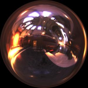
A 1998 lightprobe image of all the light falling into one spot in Grace Cathedral, San Francisco.
By Paul Debevec ( https://www.pauldebevec.com/Probes/ )

Prior to NeRFs, radiance field rendering was performed by constructing multiple local radiance fields and then blending nearby radiance fields to synthesize novel views.

A 2019-vintage pre-NeRF Radiance Field render (LLFF, https://bmild.github.io/llff/)
From https://www.matthewtancik.com/nerf

What’s a Neural Radiance Field (NeRF)?

Coming on the scene around 2020, Neural Radiance Fields (Ben Mildenhall, Pratul P. Srinivasan, Matthew Tancik, Jonathan T. Barron, Ravi Ramamoorthi, Ren Ng) are an implementation of Radiance Fields using Deep Neural Networks to render. The process of generating the NeRF is the process of training the Neural Network. It can be fairly compute-intensive to train, and there is no “one right answer”. You can keep optimizing and training and looking for a better solution that produces a better error metric than what you already have, but at some point you need to call it good enough. Backpropagation is used to push improvements back into the network.

Wikipedia explains “The network predicts a volume density and view-dependent emitted radiance given the spatial location (x, y, z) and viewing direction in Euler angles (θ, Φ) of the camera. By sampling many points along camera rays, traditional volume rendering techniques can produce an image.” So, basically, you can input an XYZ location and orientation of a ray, and the network says “about this much of that color light will come to you along that ray”, much like a conventional non-neural reverse ray-tracer or ray-marcher.

However, rather than using conventional trigonometry to solve for the light output of a given ray, you must run a deep neural network. So, this technique can be quite slow, even with fast GPU hardware. A variety of techniques have been implemented since 2020 to optimize the problem and make the rendering process faster, and also to improve/speed the training process, but NeRFs are still fairly slow. They also, like other generative neural network techniques, can “hallucinate” data – if real data isn’t available for a given view, some fictitious (plausible or not) data may be inferred by the network. This can be both good and bad – it can help fill in for missing inputs, but it also can create artifacts and anomalies.

The secret sauce that turned Local Radiance Fields into NeRFs is the thought that the concept of a holistic unified radiance field is pretty hairy. Instead of trying to solve it by devising a method for merging multiple Local Light Fields, we can construct a differentiable model with an error metric. Then we can throw a lot of compute power at the problem to let machine learning stumble forward with some gradient descent guidance until it finds and acceptable single solution.

The 2020 NeRF paper Github code repository is here.

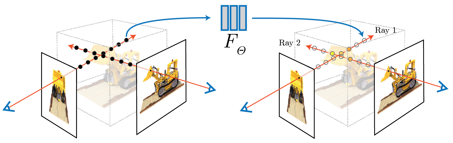
Ray Tracing a Neural Radiance Field of a Lego building block toy bulldozer.
From Representing Scenes as Neural Radiance Fields for View Synthesis

Ok, for comparison, what is Photogrammetry?

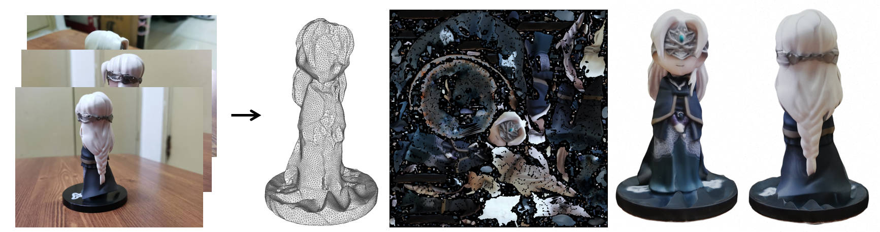
Photogrammetry is a related technique that predates NeRFs and Gaussian Splats. Like NeRFs and Gaussian Splats, it’s the process of taking multiple views from camera images, and reconstructing a scene representation. It does this by correlating camera locations and poses, identifying common visible features and reverse projecting pixel coordinates out into real-world space to see what spot a feature would need to be in to be visible in the pixel locations it was observed at.

The photogrammetry process was developed long ago but came into its own for map-making from aerial photos in the WW1 era. Many United States Geologic Survey contour maps were produced by well-dressed men standing at photogrammetry desks, adjusting the focus and alignment of two airphoto prints until only a thin area of elevation was aligned and focused, and then tracing the contour of that elevation around the map. See DEVELOPMENT OF PHOTOGRAMMETRY IN THE U. S. GEOLOGICAL SURVEY, page 7.

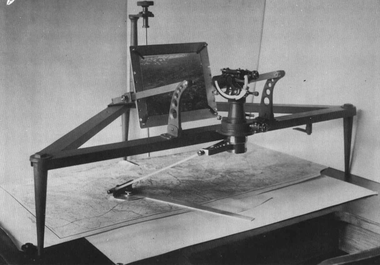
1932 model Wilson photoalidade, used to trace photogrammetry contour lines. USGS

In the modern, digital age, computer photogrammetry identifies common features scenewide, using a feature-description-vector method like SIFT or SURF, then compares features visible in every image to find common features. These common features are combined with prior knowledge of the camera+lens (often from the EXIF data in digital photos, combined with a camera+lens reference database) to compute where the camera was located when each photo was taken, and then where each identified feature was in front of the cameras. A “sparse point cloud” is created, consisting of the many thousands of locations in the scene that could be matched up in enough camera’s views to predict where that point was in the real world. Those points are also each assigned a single color (based on statistical analysis of all the colors each seemed to show in various input images). This process is now often referred to as Structure-from-Motion (SfM), as it is often done on frames from video from moving cameras, and it infers the structure of the scene geometry from the multiple-viewpoint side-effects of the camera in motion.

Once a sparse point cloud is created, a “densification” process is performed that tries to infer additional matching colored points between the sparse points. A densified point cloud can be output at this stage, and further work can be performed to group points in a common plane together into facets that are then output as triangular polygons, each with a small patch of raster texturing covering the polygon. This is called triangulation and texturing.

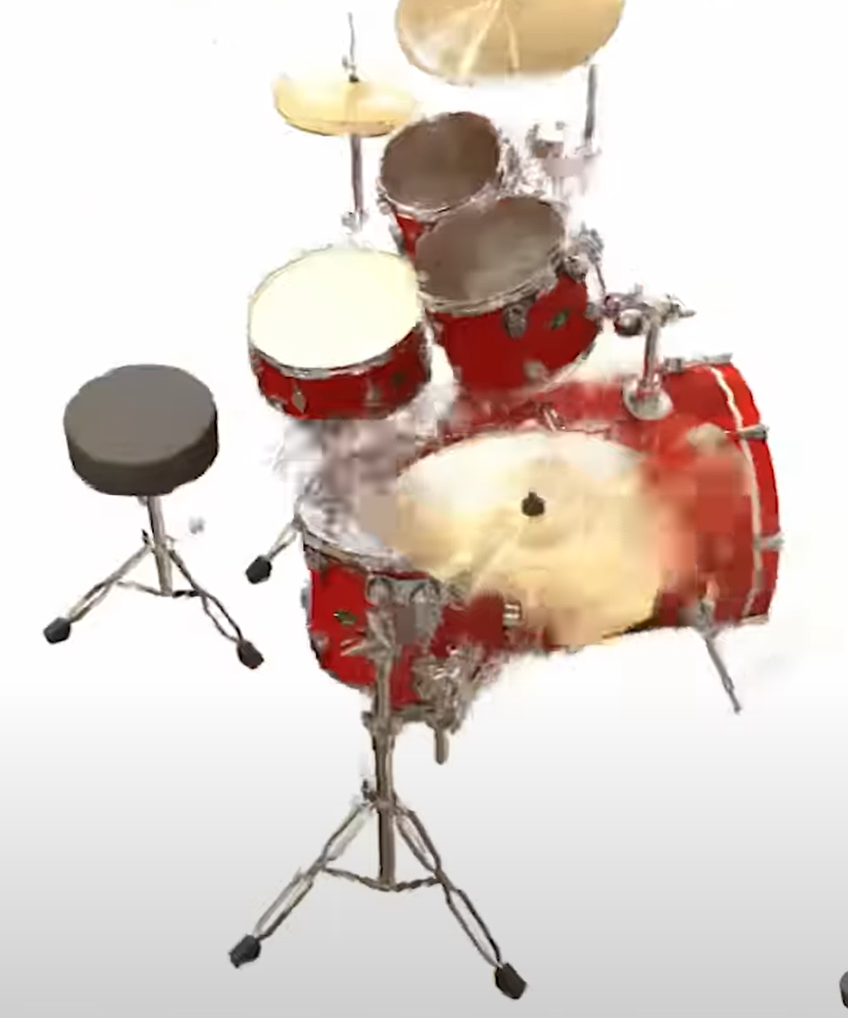
These polygons are generally opaque and hard-edged and are only created where the algorithms have a high probability of believing a piece of solid matter existed in the real world at that location. If polygons are created at less-high-probability locations, the scene tends to fill up with jagged, spiky, unwanted junk polygons that get in the way and look ugly. The downside is that sparse geometry, like organic structures such as vegetation or hair, and synthetic surfaces like metal and glass, don’t survive well through the photogrammetry and triangulation process.

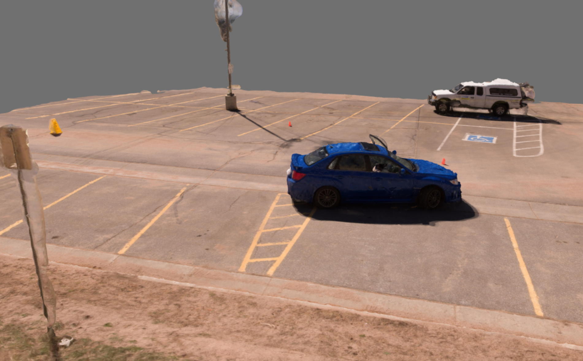
Polygonal Photogrammetry Output. Note issues with thin or transparent objects.
By the author, Chris Hanson

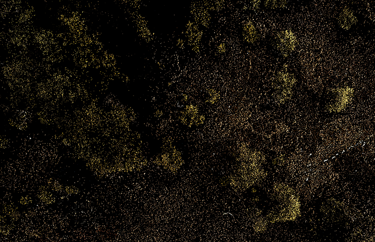
A dense point cloud of a forest, viewed from above.
By the author, Chris Hanson.

Photogrammetry CAN produce VERY good results under the right, limited conditions. There are a great number of 3D assets in the geospatial world (like 3d buildings, and 3d models in game toolkit asset stores) that are carefully produced with photogrammetry and have excellent quality.

What are Gaussian Splats and why were Gaussian Splats Invented?

As Lightning McQueen is fond of saying, Speed.

NeRFs are rendered by executing a deep neural network. While this process IS accelerated by GPUs, it’s still pretty slow. Though optimizations were being invented, in 2023 some guys at INRIA (National Institute for Research in Digital Science and Technology) in France came up with a novel approach (the INRIA SIGGRAPH 2023 paper “3D Gaussian Splatting for Real-Time Radiance Field Rendering”) for computing and storing a Radiance Field without the whole deep neural network. Their idea was to use Gradient Descent optimization, just like is used in training a Neural Network, but instead they would use a common and fast method (rasterized Gaussian Splats) of putting the radiance into pixels.

To perform the view-dependent appearance trick, they would texture each of these splats with a Spherical Harmonic representation of the radiance (color and intensity of light) emitted from that location. Both of these are FAR more efficient than the heavy lifting of running a deep neural network, and they can be easily coded in GPU shader fragment languages like OpenGL/GLSL, HLSL and similar. This technique can leverage the high-performance graphics pipelines already tweaked and optimized to death by the existing games and visual simulation software industries.

The 2023 SIGGRAPH INRIA Gaussian Splats Github code repository is here.

The secret sauce of Gaussian Splats came about from the realization that a rasterization rendering of a radiance field could also be made differentiable. Being differentiable is key to using an error metric to backpropagate changes (calculated by gradient descent) into an upstream model. But, instead of using gradient descent to tune a deep neural network that would be executed by a raymarcher for rendering, the Gaussian Splats training process uses some fairly simple geometrical operations on the existing splats (split, merge, scale, etc) to tune a much simpler scene representation. No neural network needed, when you’re done tuning, you can just rasterize the splats!

We’ll talk more later about how Gaussian Splats are computed/trained, as there are now many techniques.

Since summer of 2023, research and development of Gaussian Splats technology has advanced rapidly.

Gaussian Splatting vs NeRF

It’s very common to compare Gaussian Splatting with its immediate predecessor, NeRFs.

Gaussian splats offer a significant advantage over NeRFs in rendering speed and simplicity. Gaussian splatting achieves real-time performance by representing scenes as a collection of efficiently rasterized 3D Gaussians. This eliminates the need for complex neural networks and reduces computational overhead, making it more suitable for applications requiring fast, real-time interactions. The simplicity of Gaussian splats enhances interpretability and ease of implementation compared to the intricate multi-layer perceptrons used in NeRFs. A Gaussian Splat renderer can easily be written in Javascript and WebGL without any neural network code.

However, Gaussian splats also have their disadvantages. The discrete nature of Gaussian splats can lead to artifacts, such as pointy ellipsoid shapes, if not optimized properly. This method requires careful initialization and regularization to avoid issues with under- or over-reconstruction. In contrast, NeRFs benefit from the continuous representation provided by neural networks, which naturally smooths out inconsistencies and provides more robust handling of complex scenes, especially in regions with sparse data.

Both techniques capture view-dependent radiance capture, allowing for the representation of transparency, reflection and even refraction.

Gaussian Splatting vs Photogrammetry

It’s also normal to try to compare Gaussian Splatting with photogrammetry, the go-to technique before NeRFs, and still a very viable and practical graphics process.

As explained above, Gaussian splats utilize a collection of 3D Gaussians for scene representation, which enables real-time rendering through efficient rasterization techniques. This method excels in applications requiring fast processing and straightforward implementation, as it bypasses the need for complex mesh constructions.

In contrast, textured polygon photogrammetry relies on detailed mesh generation and texture mapping from photographic data, providing highly realistic and visually rich representations ideal for applications where visual fidelity of solid masses is paramount, such as virtual tours and architectural visualizations. Photogrammetry also generates a scene that can be interrogated for geometric analysis. Physics and collision can be easily run on polygonal meshes, and meshes can even be cleaned and fixed up for 3d printing.

The Gaussian Splats technique also struggles with the complexity of scenes that require continuous, smooth surfaces, as it operates on discrete points. Textured polygon photogrammetry can offer excellent visual quality for some model types under certain conditions, but it lacks view-dependent visual properties so materials that exhibit translucency/transparency, reflection or refraction do not reproduce well.

Recent techniques do allow the production of polygonal surfaces FROM radiance fields (potentially NeRF or Gaussian Splats), allowing a best-of-both-worlds hybrid solution.

Conversion of a NeRF to a Textured Mesh.
From https://github.com/ashawkey/nerf2mesh

Ok, but what, at a high level, are Gaussian Splats really all about? To summarize:

Gaussian Splats are a rendering technique for rasterizing a stored radiance field or lightfield into a realistic scene from multiple viewpoints, with good performance and visual fidelity, including view-dependent phenomena. The Gaussian Splats are typically generated from photos that represent a limited set of representative viewpoints via a training process that uses a gradient-descent machine learning optimization method similar to neural networks, but unlike NeRFs, Gaussian Splats do not involve Neural Networks. Gaussian Splats are typically faster to generate/train and render than NeRFs, with similar quality. They are similar in generation and rendering speed to Textured Polygonal Photogrammetry models, but are superior in visual quality for complex and organic scenes with view-dependent lighting.

Introduction to Gaussian Splats

This seems like a good place to end part 1. In later parts we’ll talk more about Gaussian Splats, creating Gaussian Splats, Optimizing Gaussian Splats, Rendering Gaussian Splats, View-Dependent Appearance and Spherical Harmonics, 2D (and 4D) Splats, Gaussian Splat Tools, Projects, Code and Libraries and new research and directions.

AlphaPixel solves difficult problems every day for clients around the world. We develop computer graphics software from embedded and safety-critical driver level, to VR/AR/xR, plenoptic/holographic displays, avionics and mobile devices, workstations, clusters and cloud. We’ve been in the computer graphics field for 35+ years, working on early cutting-edge computers and even pioneering novel algorithms, techniques, software and standards. We’ve contributed to numerous patents, papers and projects. Our work is in open and closed-source bases worldwide.

People come to us to solve their difficult problems when they can’t or don’t want to solve them themselves. If you have a difficult problem you’re facing and you’re not confident about solving it yourself, give us a call. We Solve Your Difficult Problems.