
In Part 1 we took the term apart. We covered what "splat" means, what "Gaussian" means, where the technique came from (radiance fields, then NeRFs in 2020, then the INRIA 3D Gaussian Splatting paper at SIGGRAPH 2023), and why anyone bothered to invent it in the first place. The one-word answer was speed. A NeRF asks a neural network to answer "what color and how much light, from this position, in this direction" millions of times per frame. Gaussian Splats replace that with a pile of fuzzy colored ellipsoids you can throw through an ordinary GPU rasterizer.
Part 1 was the what. This is the how.
The task: you have a folder of photographs of a scene, or a video you sliced into frames. You want a trained set of Gaussians that reproduces that scene from any viewpoint. Nobody hands you camera positions, nobody hands you a 3D model, and the photos don't come with a coordinate system stapled to them. You start with pixels and you end with a few million little glowing blobs sitting in 3D space. This post is about everything that happens in between.
There are two stages, and they are usually run by two completely different pieces of software. First you recover where every camera was standing and what lens it was looking through. Then you optimize a set of Gaussians until the images they produce match the photos you started with. The first stage is old, borrowed wholesale from photogrammetry. The second stage is the new part, and it is where the interesting machinery lives.
Find the cameras first (aka COLMAP and friends)
Here is the thing people skip past when they first meet Gaussian Splats. A Gaussian lives at a position in 3D space. To optimize that position by comparing renders against photos, you need to know exactly where the camera was when each photo was taken, which way it was pointed, and how it projected the world onto its sensor. None of that is in the photo. A JPEG is a flat grid of colors. The 3D information was thrown away the instant the shutter fired.
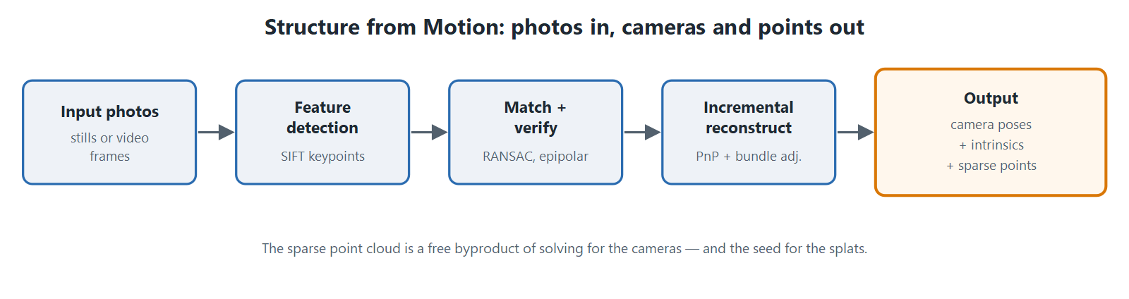
So before any splat exists, you have to reconstruct the cameras from the photos alone. The technique is Structure from Motion, universally abbreviated SfM, and it predates Gaussian Splats by decades. It is the same math that builds the sparse point clouds in classic photogrammetry, which we contrasted against splats back in Part 1. For splatting, SfM is not an optional preprocessing nicety. It is load-bearing. Get it wrong and everything downstream is quietly wrong too.
Finding the same Feature points in two photos
SfM starts by finding distinctive little patches in each image. Not edges, not flat walls, but corners, spots, texture with a recognizable local pattern. The classic detector is SIFT (Scale-Invariant Feature Transform), and although newer learned detectors exist, SIFT and its relatives are still the workhorses inside the common tools. Interestingly, SIFT is monochrome, hue and saturation value are typically discarded.
Each keypoint gets a descriptor, a vector of numbers that summarizes the pixels around it in a way that survives rotation, scale, and modest changes in brightness. The descriptor is the whole trick. It lets you take a corner of a windowsill photographed from the left and recognize it as the same corner photographed from the right, even though the raw pixels look nothing alike.
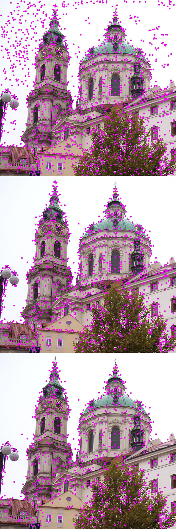 SIFT keypoints drawn as scale-and-orientation vectors. Image by Lukas Mach, licensed CC BY 3.0.
Pairwise matching, and throwing most of them away
Now you compare descriptors between pairs of images. A keypoint in image A whose descriptor is very close to a keypoint in image B is a candidate match. Do this across every pair (or, for large sets, a smart subset chosen by a vocabulary tree so you don't compare all N-squared pairs) and you get a mountain of candidate correspondences.
Most of them are wrong. Descriptors collide, repeated textures fool everything (brick walls and picket fences are notorious), and reflections are poisonous (more on them later). So the next step is geometric verification. For a pair of images, all the true matches have to be consistent with a single rigid camera motion. That constraint is captured by the epipolar geometry: the fundamental matrix if you don't know the calibration yet, the essential matrix once you do. A point in one image must lie on a specific line in the other. Matches that violate this are geometrically impossible and get discarded.
The tool that separates the good matches from the garbage is RANSAC (Random Sample Consensus). It repeatedly guesses a camera relationship from a tiny random subset of matches, checks how many of the remaining matches agree with that guess, and keeps the guess that the most matches vote for. The agreeing matches are inliers; the rest are thrown out. RANSAC is doing something that sounds like random search, we will contrast it later. RANSAC is a robust estimator for the geometry step, not the optimization method that trains the splats. Those are two different processes and it's easy to get confused here.
Triangulation
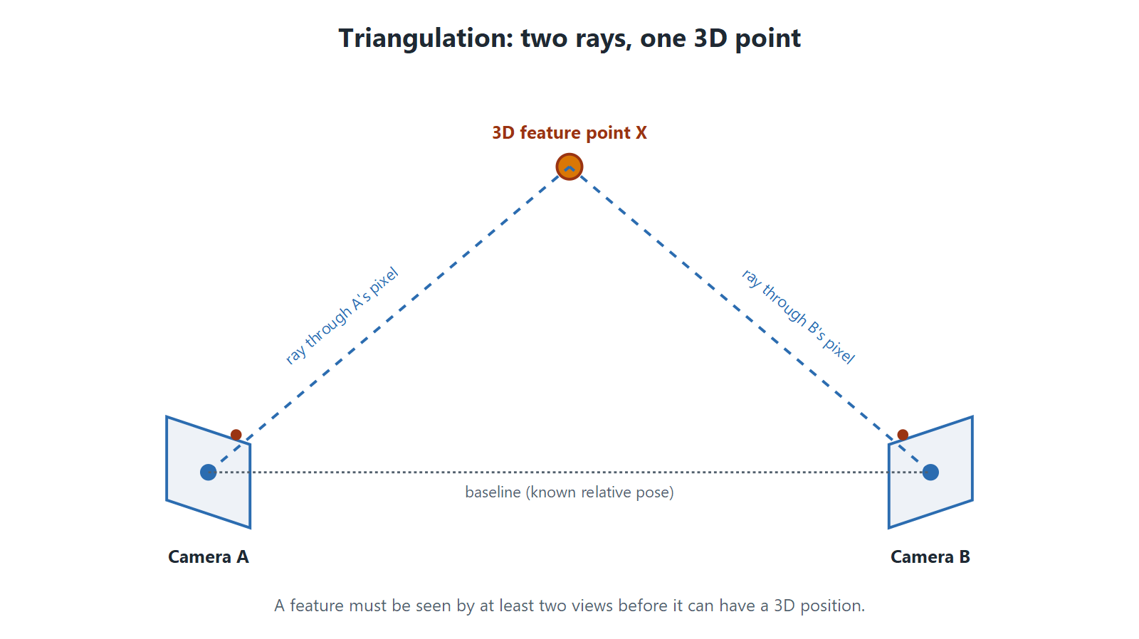
Once you know how two cameras are positioned relative to each other, and you have a feature that both of them saw, you can recover that feature's position in 3D. Draw a ray from each camera center through the feature's location on its sensor. In a perfect world the two rays cross at exactly one point in space, and that point is the feature. In the real world they nearly cross, and you take the closest approach. Triangulation is why you need at least two views of a point before it can have a 3D position at all.
Incremental reconstruction and bundle adjustment
You can't solve the whole scene at once, so the standard approach builds it up incrementally. Pick a good starting pair with a wide baseline and lots of matches. Reconstruct those two cameras and triangulate their shared points. Now find another image that sees a bunch of the points you already have. Because you know where those points are in 3D and where they landed in the new image, you can solve for that camera's position. That sub-problem is Perspective-n-Point, PnP (a stalwart of Computer Vision), and it is how each new camera gets registered into the growing reconstruction. Triangulate the new points that camera adds, then repeat. And repeat ad nauseum.
If that were all, error would pile up. Every triangulated point has a little error, every registered camera has a little error, and adding cameras one at a time lets those errors drift until the far end of the reconstruction bends away from reality. The fix is bundle adjustment, run periodically as the reconstruction grows. Bundle adjustment is a big nonlinear least-squares optimization that jiggles every camera pose and every 3D point at once to minimize the total reprojection error: the distance, in pixels, between where each 3D point actually lands in each image and where the current estimate says it should land. It is the same idea as the training loop we are about to build for the splats, run on a different set of unknowns. The "bundle" is the bundle of rays converging on each camera center and the goal is to iteratively minimize the alignment error.
When it finishes, you have three things you didn't have when you started, all in one consistent coordinate system: the pose of every camera (its extrinsics, meaning position and orientation), the camera calibration (its intrinsics), and a sparse cloud of 3D points. That sparse cloud is a free byproduct of solving for the cameras, and it becomes the seed for the splats.
Camera calibration is not exactly measured
The intrinsics deserve their own paragraph because people assume the camera "just knows" them. It doesn't, not reliably. Intrinsics are the focal length (how zoomed in the lens is, in pixels), the principal point (where the optical axis hits the sensor, usually near but not exactly at the center), and the lens distortion (how much the lens bends straight lines, worst near the edges of wide-angle and action-camera footage).
You can seed these from the EXIF metadata in the image files. EXIF often carries the focal length in millimeters and the sensor size, which together give a decent first guess at focal length in pixels. But EXIF can get stripped by editing tools, it is missing or wrong for cropped images, and it says nothing useful about distortion. So the pipeline doesn't trust prodived intrinsics, and treats them as unknowns to be recovered. This is self-calibration: the intrinsics are refined inside bundle adjustment alongside everything else, because the same reprojection-error objective is sensitive to getting the focal length and distortion right too. Nifty!
There is a useful assumption that makes this tractable. If all your photos came from the same physical camera with a fixed lens, they share one set of intrinsics. Instead of solving for focal length in every image independently, you solve for one focal length shared across the whole set, which is far better constrained. The common tools let you group images by camera model and share intrinsics within a group.
But, if you zoomed partway through the shoot, half your images have different intrinsics than the other half and the shared-intrinsics assumption is now a lie (like the cake). Rolling-shutter sensors (most phones, most drones) smear the geometry during fast motion because the top and bottom of the frame were exposed at different instants, so the pinhole model those tools assume is subtly wrong (usually only matters with frames extracted from moving video). And if you fed in images that were cropped or resized after capture, the principal point and focal length no longer correspond to the original sensor, so please avoid that in practice.
COLMAP and its relatives, and the video case
The de facto standard tool for all of the above is COLMAP, an open-source SfM and Multi-View Stereo package (Schönberger and Frahm, CVPR 2016). When someone says they "ran COLMAP on it," they mean they did the whole feature-detection, matching, verification, and incremental-reconstruction dance and got out camera poses plus a sparse point cloud. The original 3DGS code expects COLMAP output, and most of the ecosystem still speaks that format. There are faster relatives now, notably GLOMAP (Pan et al., ECCV 2024), which solves the reconstruction globally instead of incrementally and is dramatically quicker on large sets, plus various learned front-ends that replace the SIFT-and-match stage. They all produce the same kind of output: poses, intrinsics, points. Fortunately, GLOMAP produces COLMAP-compatible output data files that everyone can utilize.
Video complicates a couple of things and simplifies others. On the simplifying side, consecutive video frames are already ordered and only slightly different from each other, so matching neighbors is easy and reliable. On the complicating side, video hands you far too many nearly-identical frames, and processing all of them is wasted work and can actually hurt, because thousands of tiny-baseline pairs give you almost no new triangulation information while blowing up the compute. So you subsample: pull one frame every N, or better, pull frames adaptively based on how much the camera moved.
The bigger problem with video is motion blur. A blurred frame has smeared feature points, and smeared features match badly and triangulate worse. Handheld video and drone footage are full of them. The practical move is to detect and drop the blurriest frames before you even start, and to shoot at a high shutter speed if you have any control over the capture. A hundred sharp frames beat a thousand mushy ones. This is one of those places where the quality of the final splat is decided before any splatting happens, at capture time, and no amount of clever optimization later recovers detail that was never sharp in the source.
Sparse to Dense?
At this point you have a sparse point cloud. "Sparse" is accurate. It is only the feature points that survived matching and triangulation, so it is thousands to maybe a few hundred thousand points, and it is FULL of holes. Textureless regions (blank walls, clear sky, glass) produce no features and therefore no points. If you have only ever done classic photogrammetry, your instinct now is to densify. ("Luke, I am your Densify.")
Densification in the photogrammetry sense means Multi-View Stereo, MVS. After SfM gives you the cameras, MVS goes back to the images and, for essentially every pixel, tries to estimate a depth by comparing small patches across the views that can see it. COLMAP does this with PatchMatch stereo followed by a fusion step that merges the per-view depth maps into one dense cloud. The result is orders of magnitude more points, dense enough that you can mesh it into a solid surface by merging coplanar polygon facets into larger planar triangles. This is the classic photogrammetry pipeline: sparse cloud, then dense cloud, then mesh.
Gaussian Splatting does not need the dense cloud. Read that again. Gaussian Splatting does NOT need the dense cloud. The original 3DGS work initializes directly from the sparse SfM points, and it works fine. In fact the paper showed that even initializing from a random cloud of points, with no SfM structure at all beyond the camera poses, eventually converges to a decent result, just more slowly and with somewhat worse quality in sparsely covered regions. The optimization creates its own detail as it runs, as we will see, so it does not depend on MVS to hand it a dense starting geometry. Running MVS before splatting is mostly wasted time and, worse, MVS points carry their own errors that you would be baking in as a starting bias. It's like making a pie and mixing pebbles into the filling.
So when would you still run dense reconstruction? Three cases. First, if you also want a traditional mesh out of the same capture, for physics, collision, measurement, or 3D printing, all the things we said in Part 1 that splats are bad at. Second, in some hybrid pipelines that convert splats to meshes (look at MILo) or use a dense prior to regularize the geometry, particularly the surface-oriented 2D splat methods we'll get to. Third, when your image coverage is so thin that the sparse cloud has almost nothing in a region and you want to hand the optimizer a better starting point there. For the ordinary case (plenty of overlapping photos, you want a splat and only a splat) skip MVS and initialize from the sparse points.
Turning points into starter Gaussians
Now the Gaussian-specifc part begins. You have camera poses and a sparse cloud. You turn each point into a Gaussian.
A single 3D Gaussian is defined by a small handful of parameters, Let's cover those.
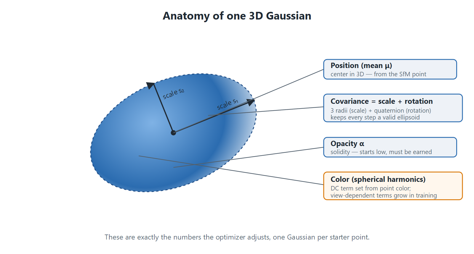
- Position (the mean): where the center of the blob sits in 3D. Initialized straight from the SfM point's location initially.
- Covariance: the size and shape of the ellipsoid. Rather than store a raw 3x3 covariance matrix, which would have to stay positive semi-definite through every optimization step or become geometric nonsense, the parameters are split into a scale (three numbers, the ellipsoid's radii along its own axes) and a rotation (a quaternion, four numbers, orienting those axes in space). Covariance is reconstructed from those as needed. This split is what keeps every gradient step producing a valid ellipsoid. It is initialized isotropic, a little round sphere (a fat point), sized from the distance to the nearest neighboring points so that dense regions start with small Gaussians and sparse regions start with larger ones to adequate cover and fill space.
- Opacity: how solid the blob is, from transparent to fully opaque. Initialized low, so Gaussians start faint and the optimizer has to prove their opacity is needed by proving they actually reduce the error metric.
- Color, stored as spherical harmonic coefficients so the color can change with viewing angle. At initialization only the constant term (the DC component, the flat average color) is set, taken from the SfM point's color. The higher-order terms that produce view-dependent shading start at zero and grow during training. Spherical harmonics get their own part later in this series; for now just know the color is a small function of viewing direction, not a single fixed RGB value.
So a starter model is one faint, round, roughly-colored Gaussian per SfM point. It looks terrible and it is supposed to. Everything good happens in the loop iteration.
Lather, Rinse, Repeat Render, Compare, Correct
The core of training is a loop, and it is conceptually simple even though the machinery inside each step is not.
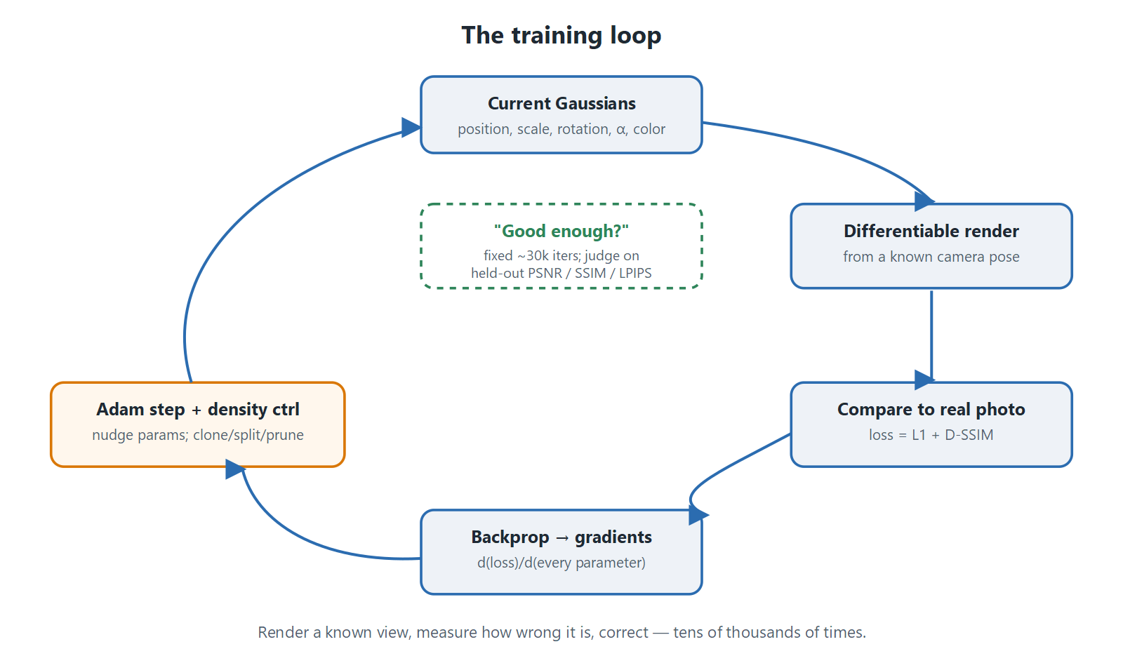
Pick one of your input photos. We know the exact camera pose for it, because SfM recovered it. Render the current set of Gaussians from that exact pose (basically, the SfM sparse point cloud, at the start). You now have two images the same size: the render and the original photo. Compare them, pixel by pixel, and compute an error metric. Use that error to nudge every Gaussian's parameters in the direction that would make the render look more like the photo. Move to another photo and do it again. Repeat tens of thousands of times.
That is the whole loop: render a known view, measure how wrong it is, and correct it, a little tiny bit. The rest of this post is about how each of those three steps works, because "measure how wrong it is" and especially "correct" are doing enormous amounts of lifting here.
The error metric, per-image and per-scene
The per-image error compares one render against one photo. The 3DGS loss is a blend of two terms. The first is a straight L1 loss: the average absolute difference between corresponding pixel colors. L1 is simple and it punishes being wrong everywhere a little. The second is D-SSIM, derived from the Structural Similarity index (SSIM), which cares about local structure, contrast, and texture rather than raw per-pixel color difference. SSIM is closer to how a human notices whether two images look alike; L1 keeps the colors on-track. The original paper weights them with a lambda around 0.2, so the loss is roughly 0.8 times L1 plus 0.2 times the structural term. That specific mix is one of the MANY knobs different methods tweak.
Each training iteration typically works on one camera at a time, chosen randomly from the set so the optimizer doesn't overfit to whatever order the photos happened to be in. The scene-wide error is just the loss averaged across all the training views. You watch the scene-wide number to know whether training as a whole is progressing; you use the per-image number to generate the corrections for that specific view.
When is it "Good enough" to stop?
People expect the loss to hit some target and the process to declare victory. That is not how it usually runs. In practice, 3DGS training runs for a fixed budget of iterations, commonly around 30,000, because the loss curve keeps creeping down with diminishing returns and there is rarely a clean threshold that means "done." The iteration budget is the stopping rule, and you just pick the budget from experience with the kind of scene you're capturing.
That said, the error metric absolutely tells you whether the result is at all good. The proper way to judge is to hold out some photos that the optimizer never trained on, render the trained splat from those held-out camera poses, and compare against the real photos it never saw. The standard scores are PSNR (a decibel measure derived from pixel error, higher is better), SSIM (structural similarity, closer to 1 is better), and LPIPS (a learned perceptual distance that correlates well with what humans call "looks right," lower is better). If the held-out scores are good, the splat generalizes to new viewpoints instead of just memorizing the training photos. If training-view error is low but held-out error is high, you have overfit, usually because you didn't have enough coverage of the scene. So the metric drives two decisions: whether to keep iterating within a run (rarely, since the budget usually governs), and whether the finished splat is actually usable or needs a reshoot [ugh].
The renderer has to be differentiable. What is differentiable anyway?
The word "correct" in the loop hides the entire secret sauce (the 11 herbs and spices AND the 23 flavors) of the technique. To nudge a Gaussian's parameters in the direction that reduces error, you need to know, for each parameter, which way to push it and how hard. That information is a derivative: how much does the final pixel error change if I wiggle this one number a tiny bit. Get that derivative for every parameter of every Gaussian and you know exactly how to adjust the whole model in one coordinated step.
This only works if the render is a smooth, differentiable function of the parameters. "Differentiable" means that if you change a Gaussian's position, or its opacity, or one of its scale values by an infinitesimal amount, the rendered pixels change by a correspondingly infinitesimal, calculable amount, with no sudden jumps. A hard-edged renderer, the kind that decides a pixel is either inside a triangle or outside it, is NOT differentiable at those edges: a tiny move flips a pixel from one color to another with no smooth in-between, and the derivative is undefined at the critical spot. You cannot compute a clean gradient through a hard edge.
Gaussians are chosen precisely because they are soft. A Gaussian has no edge. Its opacity falls off smoothly from the center to nothing, so a pixel's contribution from a given Gaussian is a smooth function of that Gaussian's position, size, orientation, and opacity. Nudge any of them and the pixel changes smoothly. That softness, which Part 1 described as the fuzzy-blob quality, is not just an aesthetic choice for pretty organic scenes. It is the mathematical property that makes the whole thing iteratively trainable.
The differentiable rasterizer that ships with 3DGS does the following, and every step of it is built so that its derivative can be computed. It projects each 3D Gaussian into the image, turning the 3D ellipsoid into a 2D ellipse on the screen (this projection is the EWA, Elliptical Weighted Average, splatting formulation, and the projection involves a linearization whose Jacobian is part of the gradient path). Don't stress if a lot of that is mumbo-jumbo, you don't need to understand it to use or implement Gaussian Splats. It sorts the Gaussians by depth. Then, for each pixel, it walks the Gaussians front to back and alpha-composites them: each Gaussian contributes its color times its opacity times how much light the closer Gaussians already blocked. That front-to-back accumulation is a smooth chain of multiplications and additions, so its derivative with respect to every input is a known formula. The implementers wrote out the analytic gradients by hand for position, scale, rotation, opacity, and the spherical-harmonic color coefficients, and that hand-derived backward pass is a large part of why the original code is fast. It runs tiled on the GPU so thousands of pixels compute their gradients in parallel.
Backpropagation is not a 90s boy band name
Once you have the error at each pixel and a differentiable path from parameters to pixels, you run that path backward. Start with how wrong each pixel is. The chain rule of calculus lets you propagate that pixel error back through the alpha compositing, back through the 2D projection, back to every parameter of every Gaussian that touched that pixel. The result is a gradient: for each of the millions of parameters, a single number saying which direction reduces the error and roughly how steeply. This backward propagation of error is exactly what "backpropagation" means, the same mechanism that trains neural networks, applied here to the parameters of geometry rather than the weights of a network.
Then you take a step. The optimizer used is Adam, which keeps a running sense of each parameter's recent gradients and adapts a per-parameter step size, so parameters with consistent gradients move confidently and noisy ones move cautiously. Different parameter types get different base learning rates, because moving a position by 0.01 and moving an opacity by 0.01 are not comparably sized changes. Take the step, and every Gaussian shifts slightly toward reproducing the photos better. Then render the next view and do it again.
This is the crux of why Gaussian Splatting works at all, and it directly answers a question people ask: why isn't this just a random search that stumbles around forever? A random walk, or a Monte Carlo method, tries changes more or less blindly and keeps the ones that happen to help. With millions of parameters, blind search is hopeless; the space is far too large to stumble into a good configuration. Gradient descent does not guess. Like a wizard, it is never early, nor is it late. At every step it computes the actual downhill direction for the error surface and moves along it confidently. Every parameter is corrected simultaneously and purposefully, using information the differentiable renderer handed it. There is stochastic flavoring, in that each step uses a randomly chosen camera rather than all of them at once, which is why it's technically stochastic gradient descent. But the direction of every step is computed, not sampled. That means the difference between rolling a scene into focus in thirty thousand deliberate steps versus never getting there with a lucky-dip search. The differentiable renderer is the thing that converts "this pixel is too red" into "move this specific Gaussian left and drop its opacity," which makes the problem solvable.
Adaptive Density Control
Gradient descent adjusts the parameters of the Gaussians you already have. It cannot, on its own, add a Gaussian where the scene needs more detail, or remove one that is doing nothing, or split an overstretched blob into finer pieces. The number of Gaussians and their coarse arrangement is a separate problem, handled by a set of heuristic rules that run periodically alongside the gradient steps. In the original work this is called Adaptive Density Control, and understanding it is understanding how a few thousand starter points become a few million well-placed Gaussians.
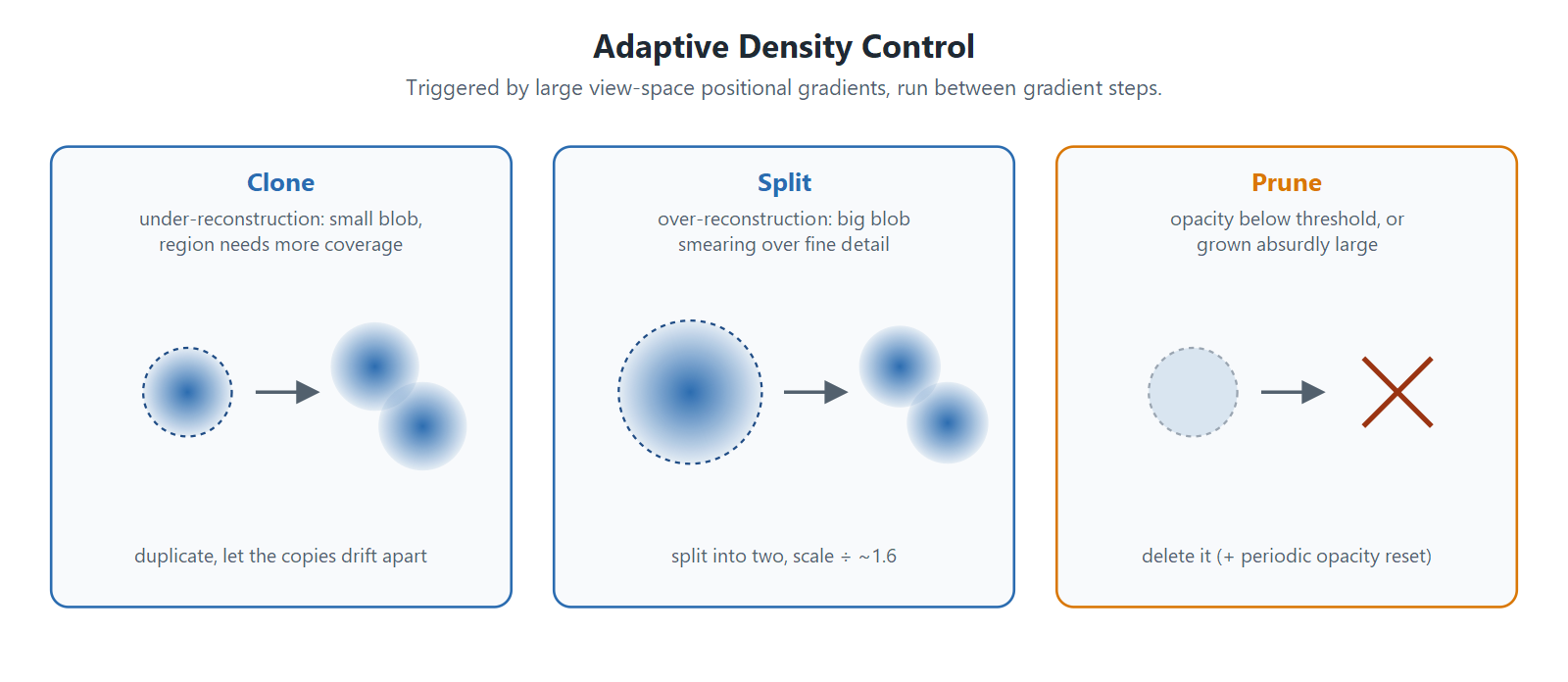
The trigger for adding Gaussians is the view-space positional gradient. If a Gaussian consistently receives a large gradient on its screen-space position, it means the optimizer keeps trying to move it to cover an area it can't adequately represent by itself. That's the signal that a region is under-described. The response depends on the size of the Gaussian:
- Clone (under-reconstruction). The region needs more coverage but the Gaussian there is small. Duplicate it, creating a second Gaussian of the same size, and let the two of them drift apart to cover the area. This grows the model into empty regions that need filling.
- Split (over-reconstruction). The region needs more detail but the Gaussian there is large, a single big blob trying to represent something with fine structure. Split it into two smaller Gaussians, dividing the scale down (the paper uses a factor of roughly 1.6), and position the children by sampling within the parent's volume. This adds fine detail where a coarse blob was smearing over it.
- Prune. Any Gaussian whose opacity has fallen below a small threshold is contributing essentially nothing and gets deleted. Gaussians that have grown absurdly large in world space, or that cover too much of the screen, also get culled, because they're usually artifacts. Pruning keeps the model from growing without bound and clears out the failures.
There is one more trick that looks strange until you see why it's there: periodic opacity reset. Every few thousand iterations, the opacity of every Gaussian is knocked back down toward transparent. Gaussians that are genuinely useful quickly re-acquire their opacity through the gradient; Gaussians that were only hanging around as vestigial near-invisible cruft, or floaters near the cameras that the optimizer was using to cheat on a few pixels, fail to recover and get pruned on the next pass. It's a controlled forgetting that stops the model from accumulating junk it can't otherwise shed.
Adaptive Densification runs during a middle window of training (after an initial warm-up, and stopped well before the end) so that the final stretch is pure refinement of a fixed set of Gaussians. The model grows, fills in, sharpens, and then settles.
And then there were many
The description above is the original INRIA recipe. It works, it's the baseline everyone cites, and it also leaves obvious room for improvement, which the field has spent since 2023 filling. The rules for when to split, clone, and prune are heuristics, and heuristics are exactly the kind of thing that different research groups tune in different directions depending on whether they care more about final quality, training speed, or Gaussian count (which drives file size and rendering cost). A few of the notable directions, without turning this into a literature review are:
- Better densification triggers. The original uses the average magnitude of the positional gradient to decide what to densify, and it systematically under-densifies some regions. Methods in the AbsGS and Pixel-GS family change what signal is measured, for instance summing the absolute gradients or weighting by how many pixels a Gaussian covers, and they recover detail the baseline misses without just carpeting the scene in more blobs.
- Anti-aliasing. The baseline renders Gaussians in a way that produces aliasing and shimmer when you zoom or change resolution away from the training views. Mip-Splatting adds a 3D smoothing filter that limits how small a Gaussian's detail can be relative to how it was sampled, plus a 2D filter in screen space, and the result holds up under zoom instead of falling apart into speckle.
- Density control as principled sampling, not heuristics. This is the direct answer to the Monte Carlo question from earlier. 3DGS-MCMC reframes the whole clone/split/prune business by treating the set of Gaussians as samples drawn from a distribution and replacing the hand-tuned heuristics with a relocation strategy grounded in that view. Note the irony: bringing an explicitly Markov-Chain-Monte-Carlo framing to the density control makes it more disciplined, not more chaotic, because the relocation is derived rather than guessed. It tends to use Gaussians more efficiently and is less sensitive to the pile of thresholds the original recipe needs you to set.
- Speed and budget. Taming 3DGS and similar work put an explicit cap on the number of Gaussians and steer densification to spend that budget where it helps most, so you can train faster and ship a smaller model, trading a little peak quality for a lot less compute and memory.
The through-line is that the differentiable-render-and-backprop core is stable and shared; what these methods change is the surrounding policy, when to add geometry, when to remove it, and how to keep it from aliasing. If you're evaluating tools or a research direction for a project, that's the axis to reason about: everyone agrees on gradient descent through a differentiable rasterizer, and everyone disagrees about the density-control rules bolted around it.
3D, 2D, and 4D splats, aren't more D's better?
We have been describing 3D Gaussians, full ellipsoids sitting in space. That is the general-purpose form and the one you'll use by default. But the dimensionality is a design choice, and two important variants change it deliberately.
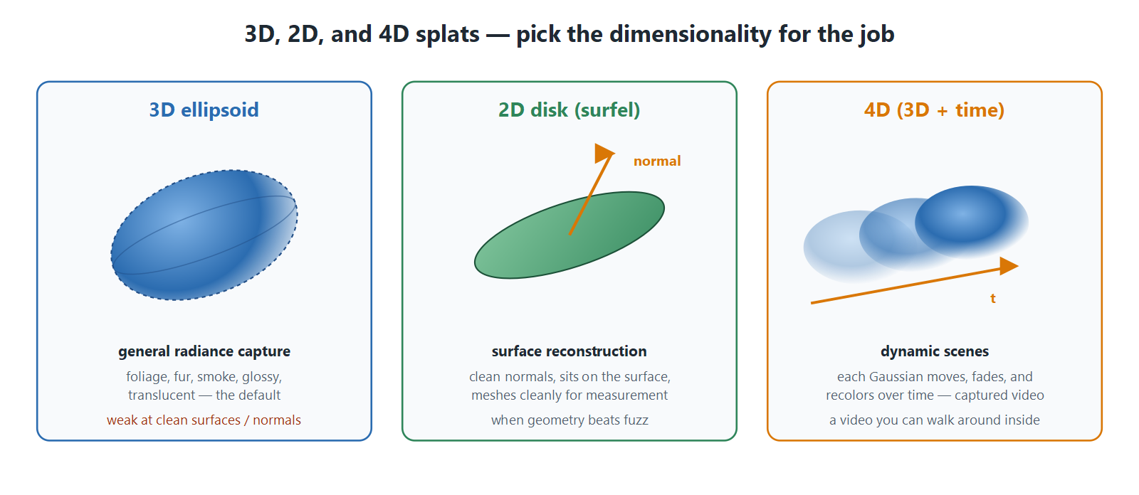
3D Gaussians are volumetric blobs. They're the right tool for general radiance capture, especially the organic and view-dependent scenes we praised in Part 1: foliage, fur, smoke, glossy and translucent materials, anything where the notion of a single hard surface breaks down. Their weakness is precisely that they're volumetric: a cloud of ellipsoids has no well-defined surface, so extracting clean geometry or accurate normals from a 3D splat is awkward, and the ellipsoids can float slightly off the true surface in ways that don't show up in a render but ruin any attempt to mesh it.
2D Gaussians (the technique usually written as 2DGS, from the 2024 work on 2D Gaussian Splatting) flatten each primitive into a disk, an oriented flat splat with no thickness, a surfel. This sounds like a downgrade and for pure image quality on fuzzy scenes it sometimes is. But a flat disk sits on a surface in a way a fat ellipsoid can't, and it has an unambiguous normal, the direction it faces. That makes 2D splats far better when the actual goal is the surface: reconstructing accurate geometry, extracting clean meshes, getting normals good enough for relighting. If we want a splat that that can also turn into a usable mesh for measurement or simulation, 2D splats are usually the best starting point, and this is one of the cases from earlier where the surface-oriented pipeline benefits from dense geometric supervision.
4D Gaussians add time as a fourth axis. A 3D splat freezes one instant in 3D like The Matrix' Bullet Time; a 4D splat represents how the scene changes over a sequence, so each Gaussian can move, rotate, grow, fade, and shift color as time advances. This is what you need for dynamic scenes: a person moving, a flag in wind, anything captured as video rather than a static set of photos of a frozen subject. The cost is more parameters, more capture discipline (you generally need many synchronized viewpoints, not one camera wandering around, because the subject won't hold still for you to walk around it), and heavier training. But it's the only way to get a free-viewpoint replay of something that was actually moving. 3D splats are a photograph you can walk around inside. 4D splats are a movie you can walk around inside.
The rule of thumb: 3D for a static scene you want to look right from any angle, 2D when you care about the surface and the geometry more than the fuzz, 4D when the subject moves.
Splat goes the weasel
So that's the full path from a folder of photos to a trained splat. SfM (usually COLMAP/GLOMAP) recovers the cameras and a sparse point cloud, and quietly self-calibrates the lenses in the process. You skip the dense MVS step that classic photogrammetry would run, unless you specifically also want a mesh. Each sparse point becomes a faint starter Gaussian. Then the training loop renders each known viewpoint through a differentiable rasterizer, measures the error against the real photo with a mix of L1 and structural loss, backpropagates that error into a gradient for every parameter, and steps every Gaussian downhill with Adam, deliberately and not by chance. Adaptive Density Control clones, splits, and prunes the Gaussians in between gradient steps so the model grows detail where the scene demands it and sheds what it doesn't use. Run that for tens of thousands of iterations and the pile of blobs snaps into a scene.
The two things we deliberately deferred are the two we'll take up next. We kept saying the color is a small function of viewing direction and waving at spherical harmonics; that's the next part, on view-dependent appearance, and it's what makes a splat's reflections and highlights track your eye the way a real surface does. After that maybe we'll build a runtime renderer itself, the part that takes a finished splat and draws it in real time in a browser or a game engine, which is a different problem from training it.
We've spent 35 years in computer graphics, and lately a good deal of it inside image-to-3D pipelines for VFX, GIS, and forensics, the computer-vision work this series grows out of. If you have a capture that will not converge, a splat you need to force into a pipeline that was never built for it, or a research direction you want evaluated before you commit real budget to it, that is the kind of difficult problem we solve. Tell us what you are working on and we will tell you straight whether splats are the right tool.
References and further reading
Illustrations in this post are original diagrams, free to reuse. The primary sources for everything above, in the order they come up:
- Kerbl, Kopanas, Leimkühler, Drettakis. 3D Gaussian Splatting for Real-Time Radiance Field Rendering, SIGGRAPH 2023. Project page · arXiv:2308.04079 · code · differentiable rasterizer
- Mildenhall et al. NeRF: Representing Scenes as Neural Radiance Fields for View Synthesis, ECCV 2020. arXiv:2003.08934
- Schönberger, Frahm. Structure-from-Motion Revisited (COLMAP), CVPR 2016. Paper · colmap.github.io
- Pan et al. Global Structure-from-Motion Revisited (GLOMAP), ECCV 2024. arXiv:2407.20219 · code
- Lowe. Distinctive Image Features from Scale-Invariant Keypoints (SIFT), IJCV 2004. Paper (PDF)
- Wang, Bovik, Sheikh, Simoncelli. Image Quality Assessment: From Error Visibility to Structural Similarity (SSIM), IEEE TIP 2004. Overview
- Zhang et al. The Unreasonable Effectiveness of Deep Features as a Perceptual Metric (LPIPS), CVPR 2018. arXiv:1801.03924
- Kingma, Ba. Adam: A Method for Stochastic Optimization, ICLR 2015. arXiv:1412.6980
- Ye et al. AbsGS: Recovering Fine Details for 3D Gaussian Splatting, ACM MM 2024. arXiv:2404.10484 · code
- Zhang et al. Pixel-GS: Density Control with Pixel-aware Gradient, ECCV 2024. arXiv:2403.15530
- Yu et al. Mip-Splatting: Alias-free 3D Gaussian Splatting, CVPR 2024. arXiv:2311.16493
- Kheradmand et al. 3D Gaussian Splatting as Markov Chain Monte Carlo, NeurIPS 2024. Project page · arXiv:2404.09591
- Mallick, Goel et al. Taming 3DGS: High-Quality Radiance Fields with Limited Resources, SIGGRAPH Asia 2024. arXiv:2406.15643
- Huang et al. 2D Gaussian Splatting for Geometrically Accurate Radiance Fields, SIGGRAPH 2024. arXiv:2403.17888
- Wu et al. 4D Gaussian Splatting for Real-Time Dynamic Scene Rendering, CVPR 2024. Project page · arXiv:2310.08528