Vision Navigation Part 2a: Implementing a Toy Vision Navigation System
Table of Contents
Part 2a: Implementing a Toy Vision Navigation System
A Navigation Map
CREDIT: Pixabay user Pexels ( https://pixabay.com/users/pexels-2286921/ )
under Pixabay Content License ( https://pixabay.com/service/license-summary/ )
Overview
So now that we’ve answered what Vision Navigation is and how it’s done, let’s look at implementing a trivial vision-based localization system and work it forward into more-sophisticated architectures capable of more ability. We’ll use OpenCV and Python.
First, we will create a completely contrived example that is the easiest and most trivial method possible to demonstrate how contextual information sampled from an image can be correlated into a localization solution. This will entail a purpose-made “environment” that literally has the position metadata encoded into the color.
2D fixed-orientation Color Gradient
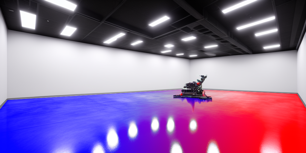
A fictional robot in a fictional Vision Navigation test chamber.
CREDIT: Created by Chris Hanson, AlphaPixel, using photos, Photoshop, and Stable Diffusion Generative AI
Imagine if you will, a rectangular room. It’s about 75 feet wide and 25 feet deep (making it a square might be too easy). Your robot wants to drive around this room, but the floor is slippery and bumpy and the magnetic field is wonky and all dead-reckoning systems and accelerometers get confused and lost. You want to introduce an absolute, vision-based navigation system to be able to tell where you are at all times. Perhaps you will even use this as a training reference for constructing an expert system or Extended Kalman Filter capable of learning how to interpret the wheel odometry and accelerometers properly so they can be of some use in the future.
For the moment we’ll ignore “outboard” vision systems that exist off the robot itself that might identify its position and communicate the information to the robot. We’ll just focus on visual sensors we could put on the robot itself, without relying on external smarts.
There are a variety of methods you could choose for encoding positional awareness into things the robot could see. For example, you could print tiny QR codes that have the position embedded in their data, paste them on the floor and have a down-looking camera spot, read and interpret them. But a simple method, and one we can simulate in a computer as a jumping-off point, would be the carefully and precisely paint the color of the floor to uniquely indicate the position at the spot being painted. So let’s turn our attention to this floor.
We need to express two different quantities in a rectangular room – the X position and Y position. Later, it might be nice to know the orientation as well as the position (together they form a combined chunk of information referred to as the “pose”). Camera-like sensors generally capture visible light in three spectra, corresponding to what humans see as Red, Green, and Blue, and turn it into numbers ranging from 0 (none of that color light) to 255 (as much of that color light as it can sense). This would represent an 8-bit (with 8 bits you can represent values from 0 to 255) RGB sensor – modern cameras can capture 12, 14 or even more bits of color depth, but 8 is sufficient for our toy problem.
With that in mind, we can use the amount of Red in the floor paint color to represent the X position within the room, and the amount of Green to represent the Y position. We don’t currently need to utilize the Blue component of what the camera sees, but we could in the future represent some other navigational information (Altitude?) with Blue. We will paint the floor with a mixture of red and blue, with no Red on the left side (look down from above) and full Red on the right, and similarly no Blue at the top edge and full Blue at the bottom. Looking down from above it will look like this:
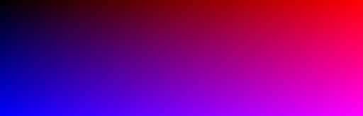
Gradient Floor Image
CREDIT: Created by Chris Hanson, AlphaPixel, using Photoshop
JavaScript Code for the Gradient Generator
					const canvas = document.querySelector('#box')
const ctx = canvas.getContext('2d')

const interpolate = (value, start, end) => (end - start) * value + start

const interpolateRGB = (value, start, end) => {
  return {
    r: interpolate(value, start.r, end.r),
    g: interpolate(value, start.g, end.g),
    b: interpolate(value, start.b, end.b)
   }
}

const calcColor = (point, topLeft, topRight, bottomLeft, bottomRight) => {
  const top = interpolateRGB(point.x, topLeft, topRight)
  const bottom = interpolateRGB(point.x, bottomLeft, bottomRight)
  const result = interpolateRGB(point.y, top, bottom)
  return result
}

const drawCanvas = () => {
  const imageData = ctx.createImageData(canvas.width, canvas.height)
  for (let y = 0; y < canvas.height; y += 1) {
    for (let x = 0; x < canvas.width; x += 1) {
      const colors = [
        { r: 0, g: 0, b: 0 },
        { r: 255, g: 0, b: 0 },
        { r: 0, g: 0, b: 255 },
        { r: 255, g: 0, b: 255 }
      ]
 const color = calcColor({ x: x / (canvas.width - 1), y: y / (canvas.height- 1) }, ...colors)
      imageData.data[(y * canvas.width + x) * 4] = color.r
      imageData.data[(y * canvas.width + x) * 4 + 1] = color.g
      imageData.data[(y * canvas.width + x) * 4 + 2] = color.b
      imageData.data[(y * canvas.width + x) * 4 + 3] = 255
    }
  }
  ctx.putImageData(imageData, 0, 0)
}

const resizeCanvas = (width, height) => {
  canvas.width = width
  canvas.height = height
  drawCanvas();
}

resizeCanvas(window.innerWidth, window.innerHeight);

window.addEventListener('resize', () => resizeCanvas(window.innerWidth, window.innerHeight))
That image is 2327×745 pixels. If we pretend that each pixel represents a 1cm spot of floor, then this is ~23m x 7m (about 75 feet wide and 25 feet deep for people who measure things in units of body parts of historic men). For now, we’re going to assume the camera has an onboard flash that perfectly illuminates the floor underneath with no color tint, and no glare. We’ll capture an image, then process it into a single-pixel value, then turn that into coordinates.
Implementing a 2D fixed-orientation Color Gradient Vision Navigation System with traditional algorithms
So let’s write some Python / OpenCV pseudocode for vision navigation in this environment. First, refer to the OpenCV camera capture example here and we’ll adapt that code (omitting some error reporting and comments for conciseness) https://docs.opencv.org/4.x/dd/d43/tutorial_py_video_display.html
					import numpy as np
import cv2 as cv
cap = cv.VideoCapture(0)
if not cap.isOpened():
    exit()
while True:
    # captures as BGR
    ret, frame = cap.read()
    if not ret:
        break
    # resize captured image to 1x1 pixels
    dim = (1, 1)
    singlePixel = cv.resize(frame, dim, interpolation = cv.INTER_LINEAR)
    # read R and G components into X and Y
    xVal = singlePixel[0, 0, 2] # third value (2) is R channel in B, G, R order
    yVal = singlePixel[0, 0, 0] # first value (0) is R channel in B, G, R order
    # turn 0-255 value range into pixel/centimeter room position coordinates
    xCoord = xVal * (2327 / 255)
    yCoord = yVal * (745 / 255)
    # for debugging, re-enlarge the frame and display it
    bigPixel = cv.resize(singlePixel, (600, 600), interpolation = cv.INTER_LINEAR)
    cv.imshow('bigPixel', bigPixel)
    print("X: " + str(xCoord) + ", Y: " + str(yCoord))
    if cv.waitKey(1) == ord('q'):
        break
cap.release()
cv.destroyAllWindows()
If you run this, and display the Gradient Floor Image (above) on a cellphone or tablet screen in front of your computer’s webcam, you can move the “floor” around in front of the “robot camera” and simulate your Python / OpenCV Vision Navigation System. You may experience some real-world problems like glare, inconsistent camera exposure, etc. We recommend trying this in a darkened room. But if you move the test pattern around in front of the camera and pretend it’s the robot moving across the floor and looking down at the gradient on the floor, you can see how a system like this might work.
The essence of the solution is capturing a camera image, averaging the entire image into one color and then interpreting that color as an X/Y position where Red encodes X and Blue encodes Y. There can only be 256 different levels of Red anywhere in the image (the image is 8 bits per channel and 256 is the highest number of combinations of 8 bits) and likewise there are only 256 variants of blue. Therefore, while there are 2327 pixels across the image and 745 vertically, the color-encoding system can only encode 256 steps in each axis. As a result, the precision of the system is limited, and it’s more limited (more than three times as imprecise!) on the X/Red axis. To decode the Red value into the X position, we need only multiply the Red value by the number of pixels per increment in Red. There are 2327 pixels (or centimeters in our ‘room floor’) across the X/Red axis, and 256 steps of Red (0 to 255), so we calculate the distance per step as 2327 / 255 (divide by 256 because we’re counting from 0 as 0 is a valid Red measurement and a valid X position). Likewise, the Y/Blue step increment is 745 / 255. You can see these scaling factors computed and used in the code above..
The BigPixel window shows the aggregate-average value of all pixels seen by the camera, and the XY coordinate readout shows the estimated position within the “room”. 0,0 is the top left where it’s black, 2327,745 is the lower right, where it’s magenta-purple. Hit the q key on the keyboard while the BigPixel window is active to exit the program.
Toy Python Vision Navigation Script with BigPixel window and coordinates displayed.
CREDIT: Created by Chris Hanson, AlphaPixel, by screen capture
Let’s elaborate a little bit, and add some better navigation display by loading the gradient floor image as a reference and plotting a marker on it.
					import numpy as np
import cv2 as cv
cap = cv.VideoCapture(0)
if not cap.isOpened():
    print("Failed to open image capture. Exiting.")
    exit()
gradient = cv.imread("XredYbluegradient.png")
if gradient is None:
    print("Failed to open reference gradient. Exiting.")
    exit()
(imageh, imagew, imagec) = gradient.shape[:3]

while True:
    # captures as BGR
    ret, frame = cap.read()
    if not ret:
        break
    # resize captured image to 1x1 pixels
    dim = (1, 1)
    singlePixel = cv.resize(frame, dim, interpolation = cv.INTER_LINEAR)
    # read R and G components into X and Y
    xVal = singlePixel[0, 0, 2] # third value (2) is R channel in B, G, R order
    yVal = singlePixel[0, 0, 0] # first value (0) is B channel in B, G, R order
    # turn 0-255 value range into pixel/centimeter room position coordinates
    xCoord = xVal * (imagew / 255)
    yCoord = yVal * (imageh / 255)
    # start with a clean copy of the reference map
    mapDisplay = gradient.copy()
    pixelCoords = (int(xCoord.item()), int(yCoord.item()))
    cv.circle(mapDisplay, pixelCoords, 5, (255, 255, 255), 2)
    cv.imshow('Vision Navigation Map', mapDisplay)
    if cv.waitKey(1) == ord('q'):
        break
cap.release()
cv.destroyAllWindows()
Now we get an intuitive Vision Navigation Map display of where our “robot” is (the white circle):
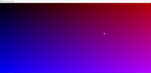
Toy Vision Navigation Absolute Position Display
CREDIT: Created by Chris Hanson, AlphaPixel, by screen capture
The accuracy of this toy project isn’t great. There are a number of things we could do to preprocess the data and improve performance, but we may do that later.
Additional Vision Navigation Functionality: Orientation from Position Derivative
What else can we do with a toy Vision Navigation system in OpenCV/Python? Wouldn’t it be nice if we could determine the orientation of our robot too?
One technique used in all sorts of navigation (not just vision-based) is referred to as Differential sampling. In the real world, if your robot used a high precision positioning system such as RTK GPS/GNSS, you can derive robot/vehicle heading by computing the position of sensors (like GPS receivers) on multiple locations on your robots and best-fitting the robot orientation to the observed sensor positions. See Attitude determination and localization of mobile robots using two RTK GPSs and IMU and High precision GPS positioning with multiple receivers using carrier phase technique and sensor fusion for some discussion.
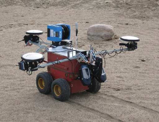
Canadian Space Agency Red Rover with three GPS antenna
CREDIT: Farhad Aghili, Alessio Salerno, © Canadian Space Agency https://www.asc-csa.gc.ca/eng/terms.asp#copyright
In our test, we will simulate this by computing the color-derived position not once for the whole image captured by the camera, but multiple times and then computing a world-space orientation vector between the computed positions.
To start, we’ll compute the position derived from a patch of pixels at the top of our camera image, and again for a sample patch at the bottom. Pretend our downward-looking robot camera has its image-space up-down axis mounted aligned with the front-back axis of the robot. A world-space vector derived from the position of the pixels at the bottom of the camera image to the calculated position of the samples from the top of the camera image will indicate the Forward direction of the robot. We’ll display this in Python/OpenCV as a line with an arrow at one end pointing to the robot Forward direction.
A small amount of organizational refactoring has been done, to make a new xyFromRGB() function to do that repetitive task. Going forward, more code could be modularized to reduce duplication.
					import numpy as np
import cv2 as cv
cap = cv.VideoCapture(0)
if not cap.isOpened():
    print("Failed to open image capture. Exiting.")
    exit()
gradient = cv.imread("XredYbluegradient.png")
if gradient is None:
    print("Failed to open reference gradient. Exiting.")
    exit()

# turn 0-255 value range RGB into pixel/centimeter atlas position coordinates
def xyFromRGB(inputR, inputG, inputB, atlasImage):
    (atlasImageH, atlasImageW, atlasImageChannels) = atlasImage.shape[:3]
    xCoord = inputR * (atlasImageW / 255)
    yCoord = inputB * (atlasImageH / 255)
    atlasXYCoords = (int(xCoord.item()), int(yCoord.item()))
    return atlasXYCoords


while True:
    # captures as BGR
    ret, capturedFrame = cap.read()
    if not ret:
        break
    # measure dimensions of captured image for subsetting
    (capturedFrameH, capturedFrameW, capturedFrameChannels) = capturedFrame.shape[:3]
    # crop out regions of interest ref https://stackoverflow.com/questions/9084609/how-to-copy-a-image-region-using-opencv-in-python
    # Crop out a section from top-center
    topCenterSubset = capturedFrame[0:int(capturedFrameH * 0.1), int(capturedFrameW * 0.4):int(capturedFrameW * 0.6)]
    # Crop out a section from bottom-center
    botCenterSubset = capturedFrame[int(capturedFrameH * 0.9):int(capturedFrameH - 1), int(capturedFrameW * 0.4):int(capturedFrameW * 0.6)]
    # resize subset images to 1x1 pixels
    dim = (1, 1)
    singlePixelTop = cv.resize(topCenterSubset, dim, interpolation = cv.INTER_LINEAR)
    singlePixelBot = cv.resize(botCenterSubset, dim, interpolation = cv.INTER_LINEAR)

    # read R and G components for top and bottom
    rValTop = singlePixelTop[0, 0, 2] # third value (2) is R channel in B, G, R order
    bValTop = singlePixelTop[0, 0, 0] # first value (0) is B channel in B, G, R order
    rValBot = singlePixelBot[0, 0, 2] # third value (2) is R channel in B, G, R order
    bValBot = singlePixelBot[0, 0, 0] # first value (0) is B channel in B, G, R order

    # turn 0-255 value range RGB into pixel/centimeter atlas position coordinates
    pixelCoordsTop = xyFromRGB(rValTop, 0, bValTop, gradient)
    pixelCoordsBot = xyFromRGB(rValBot, 0, bValBot, gradient)

    # start with a clean copy of the reference map
    mapDisplay = gradient.copy()
    # draw markers on the map
    #cv.circle(mapDisplay, pixelCoordsTop, 1, (255, 255, 255), 2)
    #cv.circle(mapDisplay, pixelCoordsBot, 1, (0, 255, 0), 2)
    cv.arrowedLine(mapDisplay, pixelCoordsBot, pixelCoordsTop, (0, 255, 0))
    cv.imshow('Vision Navigation Map', mapDisplay)
    if cv.waitKey(1) == ord('q'):
        break
cap.release()
cv.destroyAllWindows()
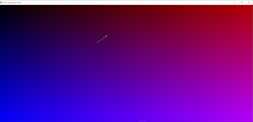
Toy Vision Navigation Absolute Position Display with Orientation
CREDIT: Created by Chris Hanson, AlphaPixel, by screen capture
Now we’ve created a super-simple toy Python implementation of Vision-based navigation using a webcam and an artificial fiducial-type landmark (the colorful “floor”) using hand-written code. In our next lesson, we’ll create the same functionality, but using a toy machine-learning implementation and then possibly grow it to a more complex machine learning model.
Where do you want to Navigate your Vision today?
AlphaPixel has experience in many different forms of computer vision navigation across numerous clients and projects. Our background in GIS and mapping, telemetry, and GPS/GNSS systems is a great fit for precise vision navigation challenges. We have numerous team members able to apply their skills and expertise to solving your difficult problems, like Vision Navigation. Need help? Smack the big green button below to get in touch with us.
Glossary
- Deep Learning https://en.wikipedia.org/wiki/Deep_learning
- Extended Kalman Filter https://en.wikipedia.org/wiki/Extended_Kalman_filter
- Feature https://en.wikipedia.org/wiki/Feature_(computer_vision)
- GPS/GNSS https://en.wikipedia.org/wiki/Satellite_navigation
- IMU/INS https://en.wikipedia.org/wiki/Inertial_navigation_system
- LIDAR https://en.wikipedia.org/wiki/Lidar
- Localization https://en.wikipedia.org/wiki/Robot_navigation#top-page
- Machine Learning https://en.wikipedia.org/wiki/Machine_learning
- Neural Network https://en.wikipedia.org/wiki/Neural_network
- Odometry https://en.wikipedia.org/wiki/Odometry
- Optical Flow https://towardsdatascience.com/understanding-optical-flow-raft-accb38132fba
- PnP / Perspective-n-Point https://en.wikipedia.org/wiki/Perspective-n-Point
- Pose https://en.wikipedia.org/wiki/Pose_(computer_vision)
- SAR https://en.wikipedia.org/wiki/Synthetic-aperture_radar
- Trilateration http://wiki.gis.com/wiki/index.php/Trilateration
- Triangulation https://en.wikipedia.org/wiki/Triangulation_(surveying)
- YOLO https://towardsdatascience.com/yolo-you-only-look-once-real-time-object-detection-explained-492dc9230006
Links, References and Jumping-off Points
- https://magpi.raspberrypi.com/articles/add-navigation-to-a-low-cost-robot
- https://bigfacerobotics.wordpress.com/2015/04/24/navigation-to-a-target/
- https://www.youtube.com/watch?v=aRzqF45j5b0
- https://www.youtube.com/watch?v=zjoYTW-tLxE
- https://paperswithcode.com/task/visual-navigation
- https://arxiv.org/pdf/2108.04097.pdf
- https://www.sciencedirect.com/science/article/abs/pii/S0967066110000808
- https://www.tandfonline.com/doi/full/10.1080/10095020.2017.1420509
